VPM

Overview

VEGAS can be used in pulsar observing modes (VEGAS pulsar modes, or VPM) that are similar to those available with the old GUPPI backend (see the GBT Observer’s Guide). VEGAS consists of eight CASPER ROACH2 FPGA boards and eight high performance computers (HPCs) equipped with nVidia GTX 780 GPUs, which together comprise a spectrometer bank (labeled A–H). VPM offers many combinations of observing modes, dedispersion modes, numbers of spectral channels, bandwidths, and integration times. Data are written in the PSRFITS format using 8-bit values.

Observing Modes

VPM can operate in one of three observing modes. All three modes can be used with coherent or incoherent dedispersion.

• search: This mode is used to record spectra with very high time resolution (typically < 100 μs) and moderate frequency resolution (> 200 kHz). It is most often used when searching for new pulsars, observing known pulsars when a timing solution is not yet available, observing multiple pulsars simultaneously, or when resolution of individual pulses is required.

• fold: This mode is used to phase-fold spectra modulo the instantaneous pulsar period. This requires a user-supplied pulsar timing solution that can be used by TEMPO1 in prediction mode (i.e., to generate “polycos”). Fold-mode is most often used for pulsar timing observations of individual pulsars.

• cal: This mode is used for polarization and flux calibration observations of the GBT noise diodes. It is actually a specialized fold-mode in which data are phase-folded at a constant frequency of 25 Hz (or a period of 40 ms). This requires that the GBT noise diodes be turned on and set to a switching period of 0.04 s (see below).

Dedispersion Modes

VPM can operate in incoherent or coherent dedispersion modes. When using incoherent dedispersion, spectra are written without any removal of intrachannel dispersive smearing, and dedispersion must be performed offline (i.e. incoherently). When using coherent dedispersion, the intrachannel dispersive delay is removed prior to detection, providing higher effective time resolution.

When operating in incoherent dedispersion modes, each FPGA and HPC form an independent spectrometer bank (labeled A–H). The center frequency of each bank can be tuned independently, and each can process a maximum instantaneous bandwidth of up to 1500 MHz, though filters in the IF system limit the maximum usable bandwidth to 1250 MHz per spectrometer bank. The center frequencies of each bank can thus be arranged to contiguously cover up to 8 x 1250 Hz = 10 GHz, though, once again, IF limitations generally limit the maximum available bandwidth from any receiver to < 4 GHz (up to 8 GHz is available for certain receivers; see here).

When operating in coherent dedispersion modes with 800 or 1500 MHz of sampled bandwidth, one FPGA sends output to all eight HPCs. Since all the HPCs are in use the maximum total bandwidth in coherent dedispersion modes is 1500 MHz, 1250 MHz of which usable. *Coherent dedispersion modes are subject to a maximum allowable dispersion measure (see below).

When operating in coherent dedispersion modes with 100 or 200 MHz of bandwidth, one FPGA sends output to one or two HPCs, respectively. In these cases, additional HPCs will not be active or write data. The exception is Bank A, which acts as the switching signal master and will always appear as active in CLEO, although it will not always write data.

Generally speaking, incoherent dedispersion is only recommended in the following use cases:

1. Blind searches for new pulsars.

2. Observations at frequencies higher than 4 GHz (i.e., C-Band), when > 1250 Hz of bandwidth is desired.

3. Observations of long-period pulsars in which very high time resolution is not needed (i.e., intrachannel dispersive delays can be tolerated).

Observations of known pulsars, especially for high-precision timing, observations of multiple pulsars with similar dispersion measures (e.g. globular cluster MSPs), and pulsar searches for which a good estimate of the dispersion measure is available should usually use coherent dedispersion.

Available VPM Modes

All configurations are subject to a maximum data rate of 400 MB/s per bank. The data rate per bank can be calculated as

\[R = 1 \,\text{byte} \cdot \frac{ n_{\text{pol}} \cdot n_{\text{chan}} }{ t_{\text{int}} }\]

where \(n_{\text{pol}}\) is the number of polarization products (4 for full Stokes parameters, 1 for total intensity), \(n_{\text{chan}}\) is the number of spectral channels, and \(t_{\text{int}}\) is the integration time (i.e. sampling time).

The following tables list all currently supported VPM modes and the vegas.scale values for each. Observers should still use the VPM Observing Tools to check the value of vegas.scale for their particular observing setup. Note that three 1500-MHz windows are used to cover the full bandwidth of the ultrawideband receiver (UWBR). The center frequency of each window is tuned such that the windows overlap by 187.5 MHz, thus ensuring continuous coverage of the full observing band. These center frequencies are 1225, 2350, and 3475 MHz. Therefore, when using UWBR, one should select the most appropriate 1500-MHz bandwidth observing mode.”

Table 18 Coherent Modes

Name	Dedispersion mode	Bandwidth (MHz)	nchan	Minimum Recommended tint (us)	Recommended vegas.scale
c0100x0064	Coherent	100	64	10.24	820
c0100x0128	Coherent	100	128	20.48	595
c0100x0256	Coherent	100	256	40.96	1650
c0100x0512	Coherent	100	512	81.92	2355
c0200x0064	Coherent	200	64	5.12	605
c0200x0128	Coherent	200	128	10.24	865
c0200x0256	Coherent	200	256	20.48	620
c0200x0512	Coherent	200	512	40.96	1720
c0200x1024	Coherent	200	1024	81.92	2430
c0800x0032	Coherent	800	32	0.64	375
c0800x0064	Coherent	800	64	1.28	420
c0800x0128	Coherent	800	128	2.56	800
c0800x0256	Coherent	800	256	5.12	940
c0800x0512	Coherent	800	512	10.24	1585
c0800x1024	Coherent	800	1024	20.48	880
c0800x2048	Coherent	800	2048	40.96	3155
c0800x4096	Coherent	800	4096	81.92	4550
c1500x0032	Coherent	1500	32	0.34133	365
c1500x0064	Coherent	1500	64	0.68267	530
c1500x0128	Coherent	1500	128	1.36533	730
c1500x0256	Coherent	1500	256	2.73067	1070
c1500x0512	Coherent	1500	512	5.46133	1450
c1500x1024	Coherent	1500	1024	10.92267	1085
c1500x2048	Coherent	1500	2048	21.84533	300
c1500x4096	Coherent	1500	4096	43.69067	3750

Attention

** Do not use longer integration times in coherent dedispersion modes. Due to the way blocks of data are sized for FFTs on the GPUs, longer integration times can result in artifacts in the final data products.**

Table 19 Incoherent Modes

Name	Dedispersion mode	Bandwidth (MHz)	nchan	Minimum Recommended tint (us)	Recommended vegas.scale
i0100x0512	Incoherent	100	512	20.48	1875
i0100x1024	Incoherent	100	1024	40.96	4010
i0100x2048	Incoherent	100	2048	81.92	550
i0100x4096	Incoherent	100	4096	163.84	990
i0100x8192	Incoherent	100	8192	327.68	580
i0200x1024	Incoherent	200	1024	20.48	1920
i0200x2048	Incoherent	200	2048	40.96	1030
i0200x4096	Incoherent	200	4096	81.92	540
i0200x8192	Incoherent	200	8192	163.84	1045
i0800x0032	Incoherent	800	32	0.64	14830
i0800x0064	Incoherent	800	64	1.28	7240
i0800x0128	Incoherent	800	128	2.56	14690
i0800x0256	Incoherent	800	256	5.12	7340
i0800x0512	Incoherent	800	512	10.24	15320
i0800x1024	Incoherent	800	1024	20.48	7495
i0800x2048	Incoherent	800	2048	40.96	14300
i0800x4096	Incoherent	800	4096	81.92	7545
i0800x8192	Incoherent	800	8192	81.92	14725
i1500x0032	Incoherent	1500	32	0.34133	14675
i1500x0064	Incoherent	1500	64	0.68267	6835
i1500x0128	Incoherent	1500	128	1.36533	13485
i1500x0256	Incoherent	1500	256	2.73067	6750
i1500x0512	Incoherent	1500	512	5.46133	13345
i1500x1024	Incoherent	1500	1024	10.92267	6655
i1500x2048	Incoherent	1500	2048	21.84533	13035
i1500x4096	Incoherent	1500	4096	43.69067	6595

Attention

Note that low bandwidth modes may be routed differently than high bandwidth modes.

• When using incoherent dedispersion and and 100 or 200 MHz of bandwidth, Bank A should be the only active bank. The exception to this rule is when using the 342 MHz feed of the prime focus receiver, in which case the IF path is routed to Bank E. Bank A will still be active because it is always the switching signal master.

• When using coherent dedispersion and 200 MHz of bandwidth, Banks A, C, and D will be active, but only bank C and D will record data. Bank A is active because it is the switching signal master.

• When using coherent dedispersion and 100 MHz of bandwidth, Banks A and D will be active, but only Bank D will record data. Bank A is active because it is the switching signal master.

The reason for this setup is that the VEGAS FPGA boards cannot be clocked at rates slow enough to natively sample 100 or 200 MHz. Instead, they are clocked at a rate of 800 MHz, but only a portion of the sampled bandwidth is sent to the HPCs for processing.

Configuring VEGAS Pulsar Modes

VPM is configured using the standard AstrID keyword/value configuration block, which is discussed in detail here. Below we review only those keywords relevant for VPM:

• obstype will always be "Pulsar".

• backend will always be "VEGAS". GUPPI has been decommissioned and is no longer installed.

• bandwidth will be either 100, 200, 800, or 1500.

• dopplertrackfreq is not always required, but it is safe to include (See Use of the dopplertrackfreq keyword Keyword` for more details). It should be equal to the center of your observing band. If you are using one spectral window (i.e., one value of the restfreq keyword) then the value of dopplertrackfreq will be equal to the value of restfreq. If you are using multiple spectral windows (i.e. multiple values for the restfreq keyword), then dopplertrackfreq should be equal to the center of the overall observing band.

• ifbw will always be 0

• tint is the integration time. Under the hood, it is controlled by the hardware accumulation length, so that tint = acclen x nchan/BW. acclen can take on values from 4 to 1024 in powers of two. If you select an integration time that does not use a power of two acclen, acclen will be rounded down to the nearest power of two (resulting in a shorter integration time). Most observers will want to keep their integration times fast enough to resolve fast MSPs, while keeping the data rate < 400 MB/s.

• swmode will either be "tp" for calibration scans or "tp_nocal" for pulsar scans.

• swper will always be 0.04.

• noisecal will be "lo" for calibration scans (this uses the low-power noise diodes) and "off" for pulsar scans.

The following keywords are VPM specific.

• vegas.obsmode controls both the dedispersion and observing mode. Allowed values are

  • "search": Incoherent dedispersion search-mode

  • "fold": Incoherent dedispersion fold-mode

  • "cal": Incoherent dedispersion cal-mode

  • "coherent_search": Coherent dedispersion search-mode

  • "coherent_fold": Coherent dedispersion fold-mode

  • "coherent_cal": Coherent dedispersion cal-mode

• vegas.polnmode controls whether full Stokes or total intensity data are recorded. Allowed values are “full_stokes” and “total_intensity”, though total intensity can only be used in incoherent search-mode.

• vegas.numchan sets the number of spectral channels. See the tables above for allowed values for various bandwidths. Care must be taken not to exceed the maximum data rate.

• vegas.outbits controls the number of bits used for output values. The only allowed value is 8.

• vegas.scale controls the VPM internal gain so that the output data is properly scaled for 8-bit values. This values are empirically measured and reccommended values are in the tables above.

• vegas.dm controls the DM used for coherent dedispersion fold and search modes. It is not used by any other modes.

• vegas.fold_parfile specifies the path to the ephemeris (parfile) used for either incoherent or coherent dedispersion fold-modes. The parfile must be compatible with the TEMPO1 prediction mode.

• vegas.fold_bins controls the number of pulse phase bins used for either incoherent or coherent dedispersion fold- or cal-modes. Enough bins should be used to fully resolve fine profile structure. Typical values are 256 in incoherent dedispersion modes and 2048 in coherent dedispersion fold- or cal- modes.

• vegas.fold_dumptime controls the length of a sub-integration in either incoherent or coherent dedispersion fold- or cal-modes. The value is specified in seconds, with 10 s being typical. It must be shorter than the total scan length.

• vegas.subband is always 1 for pulsar observing.

Experienced observers will recognize that these keywords are very similar to those used by GUPPI. This is by design. Note that the guppi.datadisk keyword has no analog in VPM. As mentioned above, GUPPI has been retired. Dual backend operation with VEGAS and GUPPI is no longer supported.

Todo

The Observer Guide has example Configurations and example scheduling blocks. Add them to the scheduling block section and reference that here.

VPM Observing Tools

Once you start observing you will want to check the quality of your data and make sure that things run smoothly. A number of tools have been designed to facilitate this, many of which are similar to those that were used for GUPPI.

The CLEO VEGAS Screen

Todo

replace Observer’s Guide reference with link to the upcoming CLEO section on gbtdocs.

Unlike GUPPI, VEGAS has its own CLEO application that can be used for spectral line and pulsar observing modes. There are two ways to launch the VEGAS CLEO application:

• From the main CLEO launcher, go to Backends and select VEGAS.

• Type cleo vegas from any command prompt.

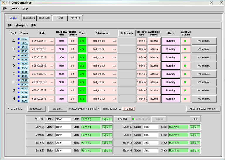
Fig. 35 This is an example of the VEGAS CLEO screen when operating in high bandwidth pulsar mode. Here VPM is configured for coherent dedispersion, so all eight banks are active and configured in the same way. However, only the power monitor for Bank A will be in use. Note the VEGAS Power Monitor button on the right-hand side. The upper panels display information about setup on individual banks. The most relevant parameters for pulsar observers are the mode and integration time. The bottom panels show the state of the VEGAS managers on each bank.

When using incoherent dedispersion, anywhere from one to eight banks may be active, depending on how the system was configured. In this case, it is completely normal for inactive banks to be configured for a different mode (possibly a spectral line mode) and/or to be in an off state. In high bandwidth coherent dedispersion modes only the FPGA on Bank A is active, but all the managers and HPCs will be used and configured in the same way. However, the power monitors on other banks will not be in use (because they are tied to the inactive FPGAs), and may not be near the target value of -20 dB (see below).

Attention

Note that in low bandwidth modes, not all banks may be active. This is normal behavior. In general, Bank A will always be active as the switching signal master, but other banks (example C and D) may be the only banks recording data. See the section on Available VPM Modes for more information.

The VEGAS Data Monitor

The VEGAS data monitor is used to check the input power levels for each bank and replaces the guppi_adc_hist tool used for GUPPI. There are two ways to launch the data monitor:

• From the VEGAS CLEO application, click on the VEGAS Power Monitor button (see Figure 1).

• Type vegasdm from any command prompt.

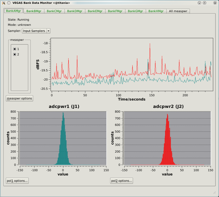
Fig. 36 This is a screenshot of the data monitor looks. Data for Bank A is selected in this example, but all eight banks are active. The chart recorder shows proper input values of approximately -20 dB. The histograms of 8-bit ADC output values are also in an acceptable range, with a FWHM of approximately 30 counts.

The top panel shows the input power level in chart recorder form for both polarization channels. The target power level is -20 ± 1.5 dB. The plot is auto-scaling, so if the power levels change (e.g., during balancing) the plot may change abruptly. Note that there are separate tabs at the top of the application for each bank, though only active banks will update. The All measpwr tab shows the chart recorder for each bank. The bottom two panels show a histogram of 8-bit values from each ADC, one for each polarization channel. These should have zero mean and a FWHM of approximately 30 counts once the system is balanced.

Note that the active banks are the same as described in the previous section for low bandwidth modes.

The vpmStatus Tool

VPM makes use of shared memory to pass configuration parameters between the managers and data acquisition programs. To check the status shared memory type vpmStatus at the command prompt while logged into one of the VEGAS HPCs. These HPCs are named vegas-hpc11 for Bank A, vegas-hpc12 for Bank B, etc. Shared memory will only be properly configured on banks that are in use.

vpmStatus plays the same role as guppi_status.

Important

Note that as of Aug 26, 2021, the VEGAS HPC names have changed. vegas-hpc1 through vegas-hpc8 should not be used. Instead, use vegas-hpc11 through vegas-hpc18.

The vpmHPCStatus Tool

When using a multi-bank incoherent dedispersion mode or coherent dedispersion mode it is useful to check the status of all the active banks at once. This is done by typing vpmHPCStatus at the command prompt of a computer on the GBO network (note: must be a RHEL7 machine). This tool displays the center frequency, status of various processing threads (network communication and dedispersion), the current data block index, and a fractional running total of any dropped packets. It also displays the last few lines from the manager logs.

Note that inactive banks may have values like “Unk” (for unknown). This may occur if those banks are configured for spectral line observing. Inactive banks also will not update during data taking. This is normal behavior. You need only pay attention to the status of banks currently in-use.

vpmHPCStatus plays the same role as guppi_gpu_status.

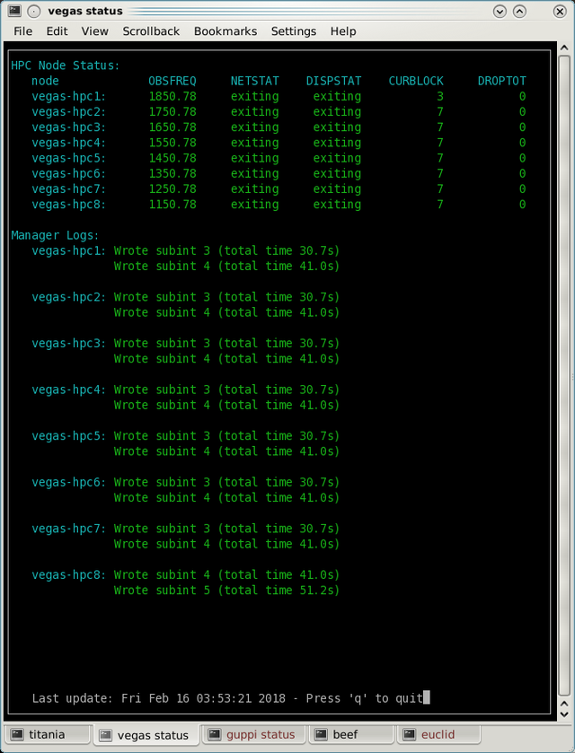
Fig. 37 This is an example of the vpmHPCStatus screen where VEGAS is configured for coherent dedispersion at L-band.

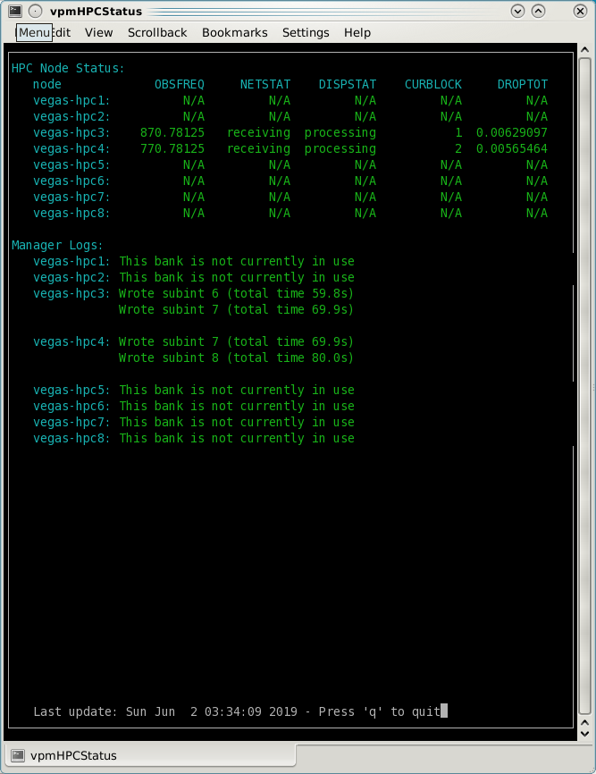
Fig. 38 This is an example of the vpmHPCStatus screen where VEGAS is configured for coherent dedispersion at at 820 MHz with 200 MHz of bandwidth.

Coherent Dedispersion VPM Data Display Webpage

Data from each HPC that is collected in coherent dedispersion fold- or cal-modes is displayed on a public webpage. The page refreshes every few seconds and should reflect the most recently written scan in close to real-time. The source name and modification time are displayed at the top of the page. The first column shows observing frequency vs pulse phase summed over the entire data file. The middle column shows frequency vs pulse phase for the most recent sub-integration. The last column shows observing time vs pulse phase summed over all frequencies.

Note

• Long scans will be broken into multiple output files, and when a new file is opened the S/N may seem to suddenly drop. This is expected and the S/N should recover as more data is written to that file.

• Under certain browsers (e.g. Chrome) the page might not always automatically refresh. If VPM seems to be running but the plots are not updating, first try clearing your browser’s cache and then reopening the page. If it still is not updating ask the GBT operator to make sure that the VPM coherent dedispersion autoplotting script is still running.

• In low bandwidth modes, not all banks may be active. A text box will appear next to those banks that are not configured to record data.

This webpage plays the same role as the old GUPPI Data Display Webpage used to.

The VPM data monitoring webpage; in this case, VEGAS is configured for coherent dedispersion with 200 MHz of bandwidth at a center frequency of 820 MHz. Only two banks are active:

Fig. 39 The VPM data monitoring webpage. In this case, VEGAS is configured for coherent dedispersion with 200 MHz of bandwidth at a center frequency of 820 MHz. Only two banks are active.

Incoherent Dedispersion VPM Monitor Webpage

When operating in incoherent dedispersion mode, bandpass plots are displayed on another public webpage. The page refreshes every few seconds and so should be close to real-time. Note that there is a separate panel for each bank, but only active banks will display data. The red curve shows the mean and the blue curves show the minimum and maximum values for the current data block. The average value should be around 30-40 counts and can be adjusted using the vegas.scale parameter. The relationship is linear for incoherent dedispersion modes. This page can also be used to monitor the RFI environment.

If you wish, you can run the same tool manually for more current data. To do this, type vpmMonitor at the command prompt while logged into one of the VEGAS HPCs. VPM must be taking data at the time. Use of the webpage is preferred.

These tools play the same role as old GUPPI Data Monitor Webpage and guppi_monitor used to.

Monitoring the VEGAS Manager Output

Output from the VPM data acquisition programs (as well as the spectral line programs) is captured by the VEGAS managers and written to log files. These log files can be found in /home/gbt/etc/log/vegas-hpcN where N is the bank number, e.g. vegas-hpc11 for Bank A. You can access these files from any GBO computer. A new log is started each time the VEGAS managers are started, so type ls -tr in the appropriate directory to find the name of the most recent log. Once you have this, you can follow the output by typing tail -f <logName>, where you replace <logName> with the appropriate file name.

Users typically will not have to check the logs unless they are trying to diagnose a problem. These log files play the same role as /tmp/guppi_daq_server.log used to, but they record output for all scans, both in incoherent and coherent dedispersion mode.

Accessing Your Data

VPM data are written directly to the lustre file system, and can be accessed from any of the machines listed as lustre clients at this website (e.g. euclid or thales).

In coherent dedispersion modes data are written to

/stor/pulsar/gbtdata/<projectID>/VEGAS_CODD/<bankID>,

where

• <projectID> is your GBT project code with the session number in AstrID appended, e.g. AGBT18A_100_01

• <bankID> is the one-letter bank name (A-H)

In incoherent dedispersion modes data are written to

/stor/pulsar/gbtdata/<projectID>/VEGAS/<bankID>

File names follow the forms:

• vegas_<MJD>_<secUTC>_<sourceName>_<scanNumber>_<fileNumber>.fits (fold- and search-modes)

• vegas_<MJD>_<secUTC>_<sourceName>_cal_<scanNumber>_<fileNumber>.fits (cal-mode)

where

• <MJD> is the modified Julian date of the observation,

• <secUTC> is the number of seconds after midnight UTC at the start of the scan. It is a zero-padded five-digit integer

• <sourceName> is the source name as identified from the Antenna manager,

• <scanNumber> is the scan number within the current Astrid session, and

• <fileNumber> is the file number within the current scan (long scans are broken across multiple files to avoid any one file from being very large). It is a zero-padded four-digit integer.

Example file names are

• vegas_58150_05400_B1937+21_0001_cal_0001.fits

• vegas_58150_05490_B1937+21_0002_0001.fits

Note

This format differs slightly from GUPPI, which did not have the <secUT> element. This has been added to avoid corner cases where GUPPI file names may not be unique.

Data are recorded in the PSRFITS standard, which can be processed by all common pulsar data analysis packages (e.g. PRESTO, PSRCHIVE, and DSPSR). Data in all modes are recorded in the /lustre/gbtdatafile store.

Fold- and cal-mode data will be archived per typical GBO data archiving policies. Due to large data volumes, search-mode data will not be included in the long-term archive. Please make arrangements to move large data sets off of the lustre file system as quickly as possible. Data can be transferred over internet (preferred) or shipped on hard disks. Please contact your project friend if you need help managing data.

Timing Offsets

Each VPM mode has a different backend timing delay. To determine the timing offset for your observing mode use /home/pulsar_rhel7/bin/vpmTimingOffsets.py

Todo

Do we need an update here to point to a rhel8 script instead of a rhel7 one?

This delay accounts for delays arising from the polyphase filterbanks employed on the ROACH2’s. Because GUPPI and VEGAS have slightly different signal paths there are some additional offsets between the two backends. Empirically these are less than 1 microsecond.

Note that overlap delays in coherent dedispersion search mode are already applied to the data via a PSRFITS keyword. This was not the case with GUPPI.

Maximum Allowable DMs for Coherent Dedispersion

The size of the data buffers uses for real-time coherent dedispersion impose a limit on the maximum allowable DM for coherent dedispersion modes. The exact maximum DM depends on the center observing frequency, the bandwidth, and the number of frequency channels. Approximate maximum DMs for common receivers and center frequencies are given below. Note that the bandwidth and number of frequency channels for UWBR are for a single spectral window.

\(n_{\rm chan}\)	Max DM (pc cm-3)
PF342 ( \(f_{\rm ctr}\) = 350 MHz; BW = 100 MHz)
64 or 256	349.28
128	698.57
512	174.64
PF800 ( \(f_{\rm ctr}\) = 820 MHz; BW=200 MHz)
64 or 1024	2414.28
128 or 512	4828.57
256	9657.15
L-Band ( \(f_{\rm ctr}\) = 1500 MHz; BW = 800 MHz)
32	1076.16
64	2152.33
128	4304.66
256 or 4096	8609.33
512 or 2048	17218.67
1024	34437.35
S-Band ( \(f_{\rm ctr}\) = 2165 MHz; BW = 1500 MHz)
32	651.58
64	1303.16
128	2606.32
256 or 4096	5212.64
512 or 2048	10425.29
1024	20850.59
UWBR ( \(f_{\rm ctr}\) = 2350 MHz; BW = 1500 MHz)
32	24.64
64	49.29
128	98.59
256 or 4096	197.18
512 or 2048	394.36
1024	788.73

Putting it All Together

Todo

This section should probably move to the recipe section and referenced here.

In summary, a typical VPM observing session will consist of the following steps.

1. Create scheduling blocks well in advance of being scheduled. Contact your project friend if you have questions.

2. At the beginning of your observing session:

   • Launch the CLEO VEGAS and VEGAS Data Monitor applications.

   • Launch the vpmHPCStatus and/or vpmStatus tools, as appropriate.

   • Log in to a lustre client and prepare to navigate to your data output directory (the directory will only be made once data start being recorded).

   • Navigate to www.gb.nrao.edu/vpm to monitor coherent dedispersion fold- and cal-mode observations and www.gb.nrao.edu/vpm/vpm_monitor to check the bandpass for incoherent dedispersion observations.

3. Once VEGAS has configured, check that the observing mode and various parameters are set properly using the VEGAS CLEO application and the vpmStatus and/or vpmHPCStatus tools.

4. Once VEGAS has balanced, check the input power and ADC output using the Data Monitor.

5. Once you have started recording data, check your fold- or cal-mode scans using the online viewers or by accessing data directly on disk. You should also check the bandpass using the VPM monitor webpage or the vpmMonitor tool.

6. Once you have started your main science scans, keep an eye on the output data and the data-taking status using the status monitors.

7. Start processing large data sets as soon as possible after your sessions ends.

Tips and Tricks

• Before writing scheduling blocks from scratch, ask your project friend if there are any already available from other projects that might suit your needs. This minimizes the possibility of an incorrect set-up or scheduling block.

• If you are searching for pulsars or observing a new source, consider observing a well known pulsar as a test source at the start of your session to make sure that things are working properly. A cal-mode scan can also be used.

• If vpmStatus and/or vpmHPCStatus show unexpected values, the system seems to be having trouble balancing, or you experience other issues, ask the operator to cycle the VEGAS managers off/on, or do so yourself if you know how. This is usually sufficient to resolve any odd states that could arise out of a partial or incorrect configuration. If this fails, ask the operator to fully restart (stop/start) the VEGAS managers. If this still doesn’t work, ask the operator to contact the on-duty support scientist.

• The GBT noise diodes are stable over short-to-medium time scales, and a number of continuum flux calibration scans are available for common observing set-ups (this is especially true of 820 MHz and L-band NANOGrav set-ups because NANOGrav observes flux calibrators at least once a month). If you’re project requires flux calibration, consider contacting your project friend to see if appropriate calibration data already exist.

• If you are observing multiple sources with relatively short scan lengths, and the operator needs to take control for a wind-stow or snow-dump, ask if you can let the current scan finish and then use Pause to let the operator take control. Once control is released back to you, you can simply un-pause and pick up where you left off. But if the operator needs to take control immediately, abort your scan and let them take over.

Important Note on Calibration

When calibrating coherent search mode data using coherent calibration scans, the resulting fluxes must be multiplied by a factor of exactly 20 to account for a scaling factor that is applied during online processing.

Use of the dopplertrackfreq keyword

The Doppler tracking frequency impacts how the first LO is tuned. This is true even if Doppler tracking is not actually used (which is the case for pulsar observing). The dopplertrackfreq keyword does not always need to be specified. If it is not specified, the Config Tool will simply set it equal to the first value specified for restfreq. For most pulsar observations, only a single restfreq is used, so we have not generally been in the habit of explicitly specifying a value for dopplertrackfreq.

However, for VEGAS observations using multiple banks to cover a wide bandwidth, we recommend explicitly specifying a value of dopplertrackfreq that is equal to the center of the observing band.

The problem is that Config Tool was intentionally designed to remember and preserve it’s state from one configuration to the next unless a keyword is explicitly assigned a new value, or the configuration is manually reset using the ResetConfig command. Unfortunately, this behavior runs counter to what many observers expect, even experienced GBT observers.

When an observer manually specifies a value of dopplertrackfreq, this value will persist, even into the next observing session, unless a new value is specified or a ResetConfig is performed. When this happens it can cause an error in calculating which sideband sense VEGAS receives – in nearly all situations it should be lower sideband, meaning that the highest frequency is in the lowest channel. When dopplertrackfreq is incorrect, it can cause the sideband to be incorrectly labeled as upper. This reverses the frequency labeling in VEGAS. For incoherent dedispersion the labels can be corrected after the fact without any impact on data quality, but for coherent dedispersion the wrong dedispersion filter will be applied online, corrupting the data.

This only occurs for certain configuration sequences, namely when switching from a pulsar mode that specifies dopplertrackfreq to one that doesn’t (it would also happen if switching from to a spectral line mode that specifies dopplertrackfreq to one that doesn’t). Switching from a pulsar to a spectral line mode (or vice versa) will reset things so that this isn’t an issue.

There are two ways to avoid this problem:

Option 1:

• Reset the GBT configuration at the start of your observing session. It is easiest to do this by simply adding this one line to a stand-alone Astrid scheduling block and submitting it at the start of your session.

• ResetConfig()

• That’s it! Most projects will only have to do this once at the start of a session, however, if you are using multiple receivers and/or center observing frequencies with different values of the dopplertrackfreq keyword during a session, you should also run this ResetConfig() command before you submit a script with a different configuration.

Option 2:

• Modify your configuration strings to always explicitly specify a value for dopplertrackfreq. This keyword specifies the Doppler tracking frequency. Even though pulsar observers don’t use Doppler tracking, it still impacts how the IF system is set up. The value of dopplertrackfreq should be equal to the center frequency of your overall observing band. If you are only using a single value for the restfreq keyword, then use the same value for dopplertrackfreq. If you are using multiple VEGAS banks to cover a wider bandwidth by specifying multiple values for restfreq, the value of dopplertrackfreq would be equal to the center of the overall observing band.

If you adopt Option 1 then Option 2 isn’t necessary, and vice versa. Of course, there is no harm in adopting both.

Transitioning from GUPPI to VPM

See here.