Astronomer’s Integrated Desktop (AstrID)

What is Astrid?

Astrid is the primary graphical interface and control workspace for the Green Bank Telescope (GBT). It consolidates multiple applications into a single environment for the creation, editing, execution, and monitoring of scheduling blocks (SBs).

• Core Functions

  • Execute Scheduling Blocks (SBs) to control astronomical observations.

  • Monitor real-time GBT status.

  • Display live data streams from the GBT.

  • Edit SBs offline or online, with validation and save functions.

  • Allow secondary observers to monitor active sessions.

• System Integration

  • Interfaces directly with GBT Monitor & Control (M&C) software.

  • Interprets Python code in SBs to coordinate device-specific M&C programs and the Scan Coordinator.

  • Applications appear in tabbed windows within the Astrid GUI.

• Applications

  • Observation Management

    • Integrates with the Observing Management Application.

    • Edit Subtab: text editor with Python syntax highlighting, enables SB editing, validation, duplication, and saving.

    • Run Subtab: supports SB queuing and execution.

  • Data Display

    • Connects to the GBT Fits Monitor (GFM) for real-time processing of pointing and focus scans.

    • Automatically updates M&C system with derived corrections.

    • Displays raw, uncalibrated continuum data as a funciton of time.

  • GBT Status

    • Provides real-time operational data, including:

      • Local Sidereal Time (LST) and UTC

      • Observer and project ID

      • Antenna position

      • Scan and IF configuration

How to start AstrID?

Type astrid from the command line on any Linux computer in Green Bank. The first thing you will see is the AstrID “splash screen”.

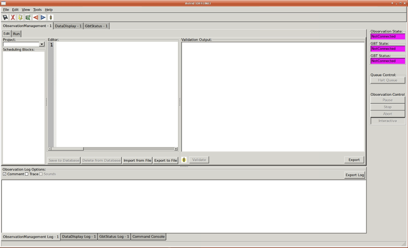
The AstrID GUI should appear on screen after 10-20s.

Astrid Modes

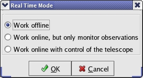
On startup AstrID will automatically ask what mode to operate in via a pop-up window.

You can reopen the selection window any time by clicking File \(\rightarrow\) Real time mode... in the AstrID GUI.

Important

You should use File \(\rightarrow\) Real time mode... to relinquish control of the telescope immediately after your scheduled observing session.

You should select the most appropriate mode for your purpose:

• Work offline

  Primarily used to create, edit and validate SBs. It is alo the preferred method to look at previously obtained data in the Data Display since online modes will continually refresh the display window with near-real time data.

• Work online, but only monitor observations

  May be used to view what is happening in the AstrID observing logs and Data Display for the current observations. You will not be able to submit SBs or affect observing in any manner.

• Work online with control of the telescope

  Use to perform observations with the GBT by allowing you to submit SBs. Log information and real-time data displays are also available in this mode.

  Note

  Working online requires the GBT operator to “put you in the gateway”, i.e. give you security access.

Table 9 AstrID mode features

Mode	Edit & Validate Syntax	Validate Configuration	Submit SBs	Observing Logs	Data Display
Offline		Simulated			Historical [1]
Online (monitor)		Simulated			Real-time
Online (control)		Real [2]	[3]		Real-time

Table Footnotes

[1]

Previously acquired data should always be viewed in offline mode.

[2]

Requested configurations are validated with respect to the actual dev_health.conf rather than the simulated “ideal” universal cabling file.

[3]

Only permitted when you are “in the gateway”, i.e. the GBT operator has given you security access

AstrID GUI Composition

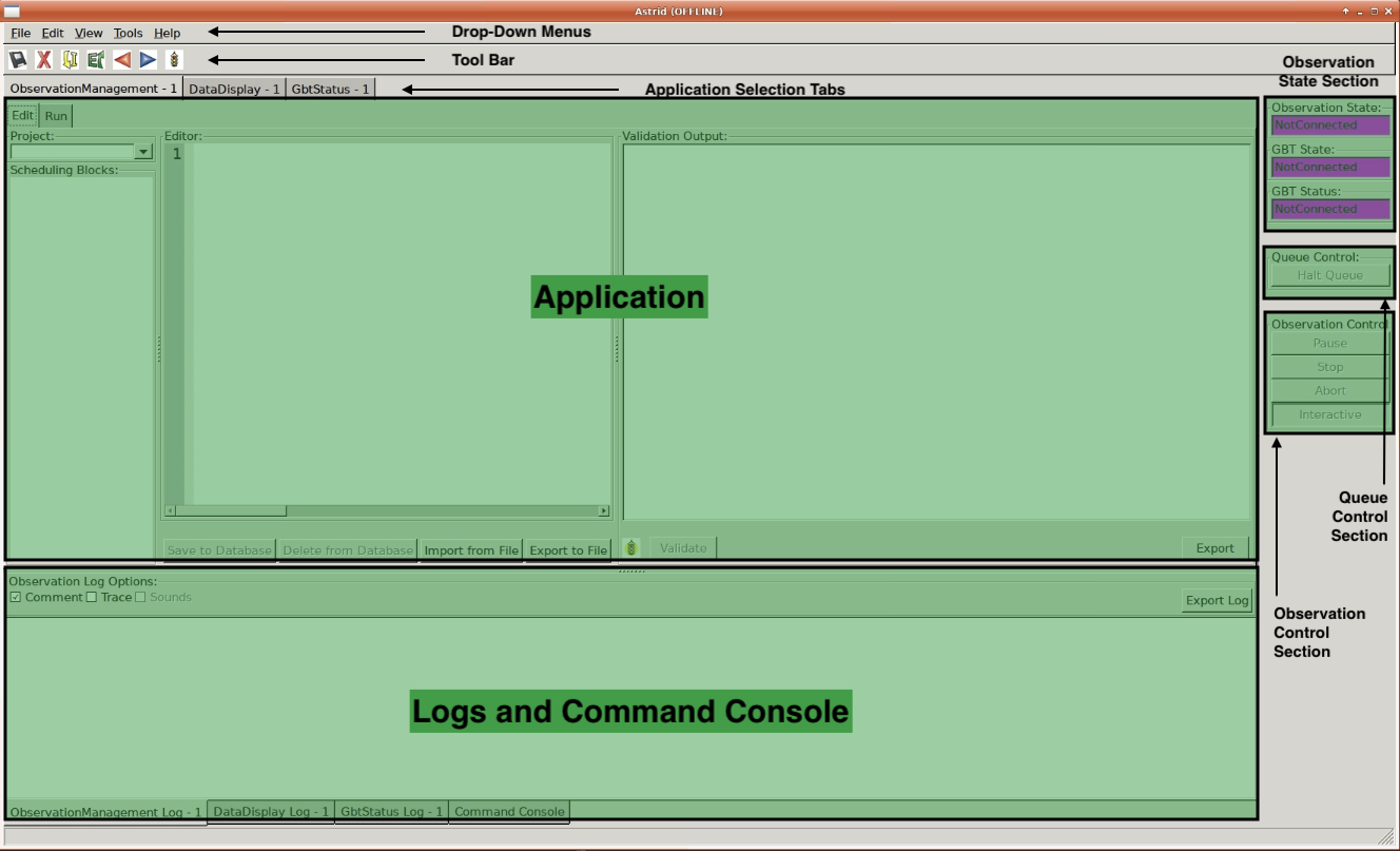
The AstrID GUI layout consists of several components:

Resizing AstrID Display Areas

It is possible to resize some of the display areas within AstrID. If you hover the mouse over the bar separating two display areas you will get a double-arrowed resize cursor. If you then hold down the left mouse button you can use the mouse to move the border and resize the display areas.

Application

This comprises the majority of the space within the AStrID GUI and shows the contents of the Application selected by the application selection tabs.

Application Selection Tabs

The application selection tabs are located under the Drop-down menus and the Toolbar The top level of tabs allow users to switch between the three main Astrid applications: * Observation Management, * Data Display * GBT Status.

Each application has its own set of subtabs.

Drop-Down Menus

In the top, left hand side of the AstrID GUI you will find the drop-down menus. The contents of the drop-down menus change according to which Application is currently being displayed on the AstrID GUI. We will not discuss all of the options under the drop-down menus in this document but we will provide some highlights.

• File

  • New Window - Launch applications within the AstrID GUI or in an independent GUI.

  • Close Window - Close the currently displayed application in the AstrID GUI.

  • Real time mode... - Change between the operational modes of AStrID.

• Edit - Standard “Windows” undo, redo, cut and paste options.

• View - Display or hide the Toolbar or view AstrID in Full Screen mode.

• Tools - Only active for the Data Display Application. You may use checkboxes to select various tooltips such as info, pan, and zoom. You can also change the “Heuristics”used during the reduction of pointing and focus observations by selecting Options....

• Help - Bring up documentation for some, but not all applications.

  Note

  The links in the documentation are outdated.

Toolbar

The Toolbar is located just under the Drop-down Menus near the top of the AstrID GUI. The contents of the Toolbar change depending on which application is being displayed in the AstrID GUI. The Toolbar options are a subset of commonly used options from the Drop-down Menus. When you leave the mouse situated over one of the Toolbar buttons for a few seconds a pop-up will appear that tells you what action the Toolbar button will invoke.

Logs

The Log Window is located in the lower portion of the AstrID GUI underneath the Application display area. Clicking on the log tabs at the very bottom of the GUI will display log information for the Observation Managament, Data Display, or GBT Status applications. Viewing a specific log will also change the application window to display the matching application.

The contents of the Observation Management application Log may be saved to an external file via the Export Log button. Note that closing or restarting AstrID will clear the Observation Management Log. If you wish to retrieve an unsaved observating log, please contact your GBT project friend.

Command Console

The Command Console is a Python shell that imports the Configuration Tool and Balance APIs. Both APIs will only interact with the Monitor & Control (M&C) systems if the user has been granted security access and is operating AstrID from the Work online with control of the telescope mode (see Astrid Modes).

State

There are three indications of state located in the upper right corner of the AstrID GUI.

• Observation State indicates AStrID’s state.

  • Not Connected: AstrID is not communicating with the M&C system (such as in its offline mode).

  • Idle: AStrID is communicating with the M&C system and no SB is currently being executed

  • SB Executing AStrID is communicating with the M&C system and an SB is running

  • SB Paused: AstrID is communicating with the M&C sstem and an SB has been paused

• GBT State indicates the M&C system state.

  • Not In Service: the M&C system is not working properly

  • Not Connected: the M&C system is not working properly

  • Unknown: the M&C system is working but does not know the state of any of the hardware devices

  • Ready: the GBT is not doing anything

  • Activating or Committed: the GBT is preparing to perform an observation

  • Running: the GBT is taking data during a scan

  • Stopping: the scan is ending

  • Aborting: the scan is ended for any abnormal reason

• GBT Status indicates the error state of the M&C system.

  • Unknown or Not Connected: the gls{MC} system is not communicating properly with the hardware

  • Clear, Info or Notice: there are no significant problems with the GBT

  • Warning: it is worth asking the Operator what the problem is, but it may not affect observation quality.

  • Error: there is potentially something wrong that may need attention

  • Fault or Fatal then something has definitely gone wrong with the observations

Queue Control Button

The Queue Control Button is located between the Observation State Section and the Observation Control Section on the right of the AstrID GUI. These buttons gives you control of the SB queue.

• Halt Queue: If this button is not activated then the SB in the Run queue will continue to be executed in order. If this button is activated it will finish the currently running SB but will not allow the next SB in the Run Queue to execute until the button is returned to its default off state.

Observation Control Button

The Observation Control Buttons are located in the lower-right of the AstrID GUI. These buttons give you control of the GBT during the execution of an SB and have the following functions:

• Pause: Pause the SB after the completion of the current sub-scan (if in progress).

• Stop: Stop the current sub-scan (if in progress) and unterrupts current SB, offering you a chance to exit the SB. This is a nice, gentle way to stop a scan.

• Abort: Abort current sub-scan (if in progress) and interrupt current SB, offering you a chance to exit the SB. This may lead to corrupted data.

• Interactive: When selected, will cause AstrID to automatically answer any pop–up query. AstrID will always choose what it deems to be the safest answer. This is useful when you have to leave the control for an extended period of time (such as when you go to the cafeteria to eat, etc.).

Observation Management Tab

The Observation Management Application consists of two sub-GUIS: the Edit Subtab and the Run Subtab. In the Edit Subtab you can create, load, save, and edit SBs. You can also validate that the syntax is correct. The Run Subtab is where you will execute GBT observations.

The Edit Subtab

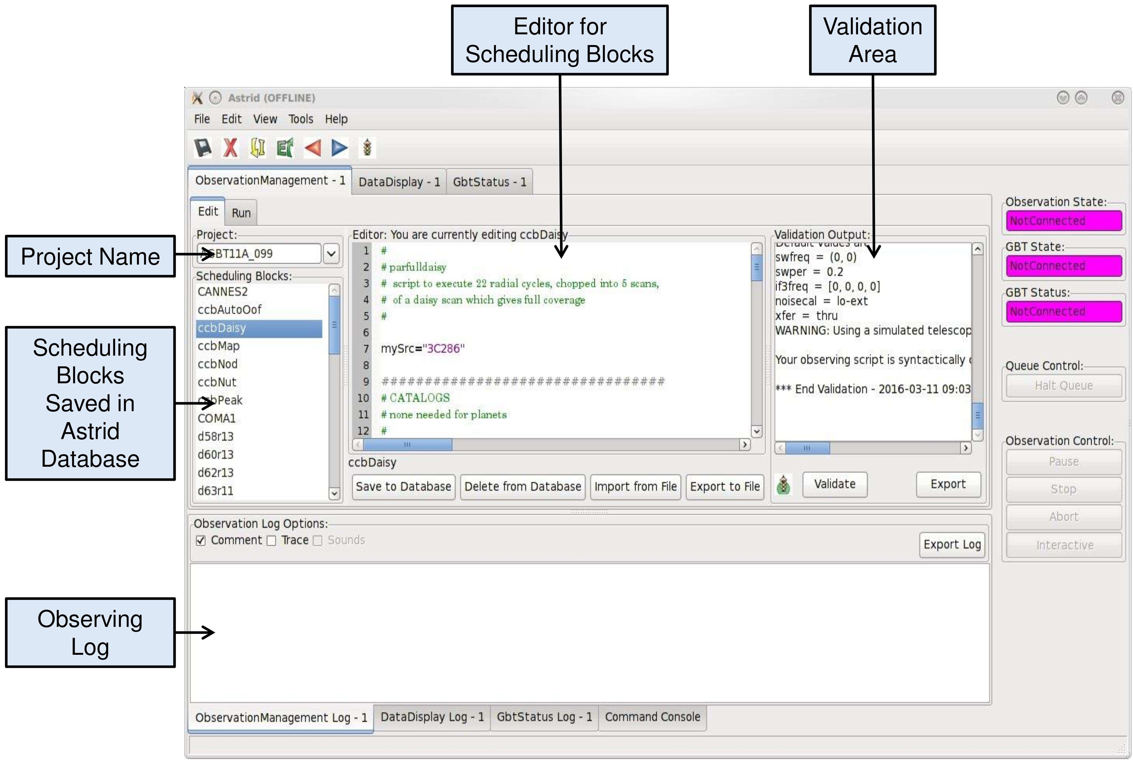
The Edit Subtab has five major areas: a list of Project Names, SBs that have been saved into the AstrID database for that project, an editor, a validation area, and a log summarizing the observations.

You can find detailed information on the content and creation of SBs here.

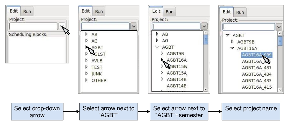
Project Name and List of SBs

To access scheduling blocks associated with your project, you will need to enter your Project Name in the Project window located in the upper left part if the Edit Subtab. Your Project Name is the code that your GBT proposal was given with the prefix AGBT, e.g., AGBT16A_001. To enter a Project Name you may either type it in directly, or use the drop-down arrows to navigate to your project through a project hierarchy as shown here:

After doing this you will see in the window labeled Scheduling Blocks a list of SBs, if any, that have been previously saved into the AstrID database. If an SB has been validated (i.e. it is syntactically correct) then it will appear in bold-face type. This means that it can be executed. If a script has been saved but is syntactically incorrect it will appear in lighter-faced type and cannot be executed.

Editor

You can use the Editor to create or modify an SB within AstrID. Standard Windows functions like Ctrl-X (to cut selected text), Ctrl-C (to copy selected text), and Crtl-V (to paste selected text) can be used within the editor. The editor lists the line number on the left hand side of the window and marks Python code as follows:

• Green highlighted text - Commented characters

• Black highlighted text - Standard Python commands/syntax

• Purple highlighted text - Strings

• Magenta highlighted text - Triple quoted strings (used in Python to enclose strings that span multiple lines)

• Dark blue highlighted text - Python functions

• \(\boldsymbol{\ominus}\), \(\boldsymbol{\oplus}\) - Marks the start of an indented block of Python code such as an if statement or for loop. Clicking on \(\ominus\) will collapse the indented code block and change the symbol to \(\oplus\). Likewise, clicking on \(\oplus\) will expand a previously collapsed code block.

The editor also has four operational buttons:

• Save to Database - This button will check the validation of the current SB and then save it to the AstrID database. A pop-up window will notify you if the SB did not pass validation. A second pop-up window will allow you to set the name that the SB will be saved under in the AstrID database.

• Delete from Database - This button will delete the currently selected SB from the AstrID database.

• Import from File - This button will allow you to load an SB from a file on disk.

• Export to File - This button will allow you to save the edited SB displayed in the editor to a file on a disk. This does not save the SB into the AstrID database.

The first time you select either of the Import from File or Export to File buttons you will have a pop-up window that lets you select the default directory to use. After selecting the default directory you will get a second pop-up window that shows the contents of the default directory so that you can select or set the disk file name to load from or export to.

Adding and Editing SBs in the Database

• Saving a Scheduling Block to the Database

  If you have already created an SB outside of AstrID, you should go to the Edit Subtab in AstrID and then use the Import from File button to load your SB into the Editor. Alternatively you can just create your SB in the Editor. To save the SB into the AstrID database you just need to hit the Save to Database button. This will trigger a validation check on your SB and then a pop-up window will appear which allows you to specify the name which you would like to use in the list for your SB.

• Selecting a Scheduling Block

  If you perform a single click on any SB in the Scheduling Block list, the contents of the selected SB will appear in the Editor. The selected SB will be highlighted with a blue background.

• Mouse-button Actions on the selected Scheduling Block

  If you perform a right mouse button click on the selected SB a pop-up window will appear that will let you rename, create a copy or save the SB to the AstrID database. You can also delete the SB from the AstrID database. You may also rename the SB if you perform a left mouse button double click on the script name in the list.

Validator

The validation area is where you can check that the currently selected SB is syntactically correct. This does not check for run-time errors and thus, does not guarantee that the script will do exactly what you want it to do. For example, it cannot check that you have the correct coordinates for your source. You will also see error messages, notices and warnings from the validation in this area.

The validator will attempt to verify that you are using a legal configuration. When run in AstrID’s offline mode, the validator can only compare your requested configuration with a simulated “ideal” model of the telescope hardware. To perform a full configuration check against the true hardware state of the telescope (modelled by the dev_health.conf file), you must be running AstrID from the Work online with control of the telescope mode.

Before an SB can be run within AstrID it first must pass validation. To validate a script without saving it you can just hit the Validate button. An SB automatically undergoes a validation check when you hit the Save to Database button in the editor. Any messages, etc. from the validation will appear in the “Validation Output” test area. You can export these messages to a file on disk by hitting the Export button in the validation area.

The state of an SB’s validation is shown by the stop-light left of the Validate button. If the script has never been validated or has been changed since the last validation the stop-light will have the yellow light on. If the SB fails validation the stop-light will turn red, while it will turn green if the SB passes validation.

Note

for-loops with many repeats can take an extended amount of time to validate since the Validator will go through each step in the loop. Also be careful of infinite loops in the validation process. Use of time functions such as Now() always return None in the validation.

The Observing Log

The observing log is always visible at the bottom of the Observation Management Tab. It shows information from the execution of SBs in either of the AstrID online modes. The observing log can be saved to a disk file by hitting the Export button that is just above the top right corner of the log display area. Note that closing AstrID will clear the observing log. If you wish to retrieve unsaved observing log information, please contact your GBT project friend.

The Run Subtab

In the Run Subtab you can queue up SBs to perform the various observations that you desire to make. The Run Subtab has five components. Across the top of the Run Subtab you enter information that will be put into the headers associated with the observations. On the left is a list of SBs that you can execute. On the right are the “Run Queue” which holds SBs that are to be executed in the future, and the “Session History” which shows which SBs have previously been executed. At the bottom is the “Observing Log”.

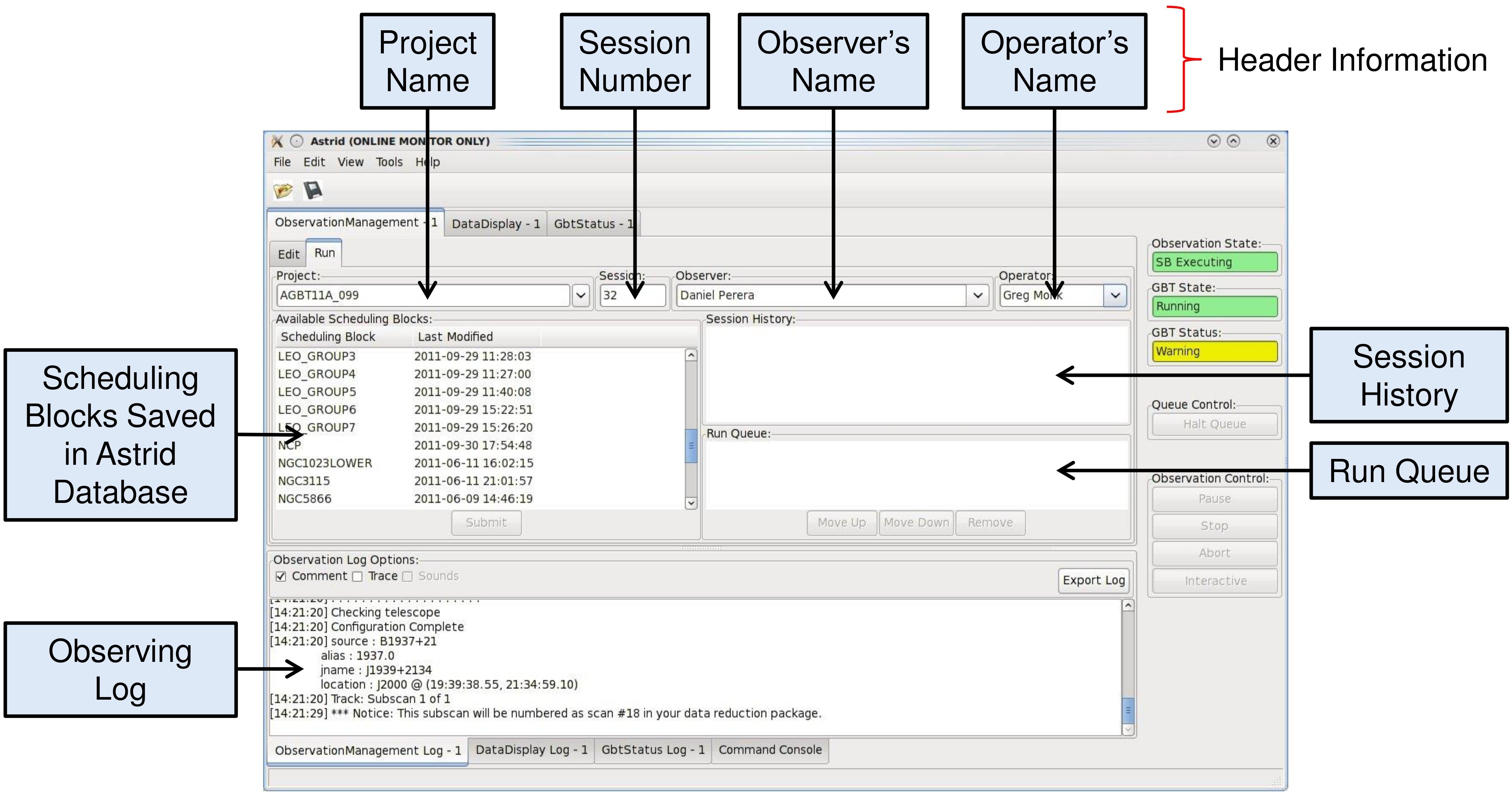
Header Information Area

The following fields must have entries before an SB can be executed:

• Project:

  Just as in the Edit Subtab you use the drop-down menu to select your Project Name. If your project is not listed, ask your GBT project friend or the telescope Operator to add it to the database.

• Session:

  A session is a contiguous amount of time (a block of time) for which the project is scheduled to be on the telescope. Each time a project begins observing for a new block of time it should have a new session number. The session number is usually determined by AstrID and automatically entered. However, there are cases (such as AstrID crashing) where the session number could become incorrect. You can type in the correct session number if needed.

  Note

  A “session” in AstrID is equivalent to an “observing period” in the lingo of the DSS. The word “Session” has a different meaning in the DSS.

• Observer’s Name:

  This is a drop-down list where you choose the observer’s name. Only the PI on a project are guaranteed to have their name in this list. If your name is not listed, ask your GBT project friend or the telescope operator to add it.

• Operator’s Name:

  This is a drop-down list from which you pick the current operator’s name at the beginning of your observations.

Submitting an SB to the Run Queue

In order to execute an SB you must:

1. Be in the Work online with control of the telescope mode.

2. Be in the gateway (contact the operator).

3. Select the Observation Management Tab.

4. Select the Run Subtab.

5. Make sure that the header information fields all have entries.

6. Select the SB you wish to execute from the list of available SBs.

7. Hit the Submit button below the list of SBs.

Your SB is then automatically then sent to the Run Queue.

Note

Double-clicking on an SB is the same as selecting the SB and then hitting the Submit button.

The Run Queue and Session History

When an SB is submitted for execution it is first sent to the Run Queue. This contains a list of submitted SBs that will be sequentially executed in the future.

When an SB begins execution it is moved to the Session History list. So the Session History list contains the currently executing SB on the first line and all previously executed SBs that have been run while the current instance of AstrID has been running on subsequent lines.

If there are not any SB in the Run Queue when a new SB is submitted for execution it may appear that the SB just shows up in the Session History. However it has indeed gone through the Run Queue - albeit very quickly.

The Observing Log

The observing log is always visible at the bottom of the Observation Management Tab. It shows information from the execution of SBs. The observing log can be saved to a disk file by hitting the Export button that is just above the top right corner of the log display area. Note that closing AstrID will clear the observing log. If you wish to retrieve unsaved observing log information, please contact your GBT project friend.

Data Display Tab

The Data Display Tab provides a real time display of your GBT data so that you can check that you are getting valid data. The Data Display is actually running an application called GBT Fits Monitor (GFM). This application provides scan-based display and analysis of GBT data, either in real-time as the data is being collected, or in an offline mode where it can be used to simply step through the scans from an observation. You are encouraged to run GFM offline for reanalyzing data during observations. A separate GFM application can be launched from the Linux prompt via the gfm command or AstrID could be switched to offline-mode.

Working Online

If you are using either of AstrID’s online modes (see Astrid Modes) and have selected the DataDisplay tab, then the data display will update as new data are obtained. Continuum and Spectral Line data are only updated when these displays are being viewed.

Important

Pointing and Focus data are always automatically updated whether or not their displays are being shown or not. Due to this feature, clicking on previous observations while Pointing and Focus scans are in progress can confuse GFM and should be avoided.

The list of scans will always automatically update.

Working Offline

You can look at data that have already been taken with the GBT by running AstrID in offline mode. To view data in this mode you need to follow these steps:

1. Change the AstrID mode to offline (see Astrid Modes).

2. Select the DataDisplay tab in AstrID

3. Select File \(\rightarrow\) Open from the drop-down menu or click the icon in the toolbar.

4. Select a project ID from the list of project directories in /home/gbtdata/.

5. Double-click ScanLog.fits file to access the data.

   Note

   It may take several seconds to a few minutes to access all of your scans depending on the amount of data to load. The process is complete when you see a list of scans displayed sequentially on the left hand side of the GFM display.

6. Click on a scan in the scan list window to process it.

Pointing and Focus Data Display

Pointing scans (from Peak(), AutoPeak() and AutoPeakFocus()) will appear under the Pointing Tab. If working online, the data display will automatically process the pointing scans.

Note

Clicking on previous scans while Pointing and Focus scans are in progress may interfere with automatic processing.

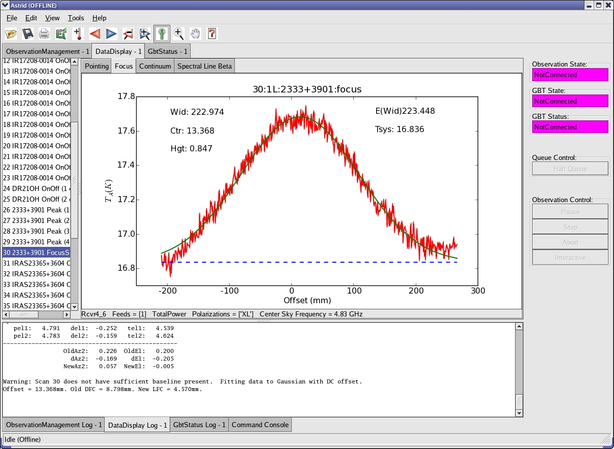
It will calibrate the data, remove a baseline and fit a Gaussian to the data. After the two azimuth scans (cross-elevation, i.e. \({\text{Az}} \times \cos{({\text{Dec}})}\)) it will then automatically update the GBT M&C system with the new azimuth pointing offset values that it determined. It will then automatically update the elevation pointing offset after the two elevation scans, unless certain criteria are not met (see Fitting Acceptance Options). Here is a sample of the Data Display Application after a pointing

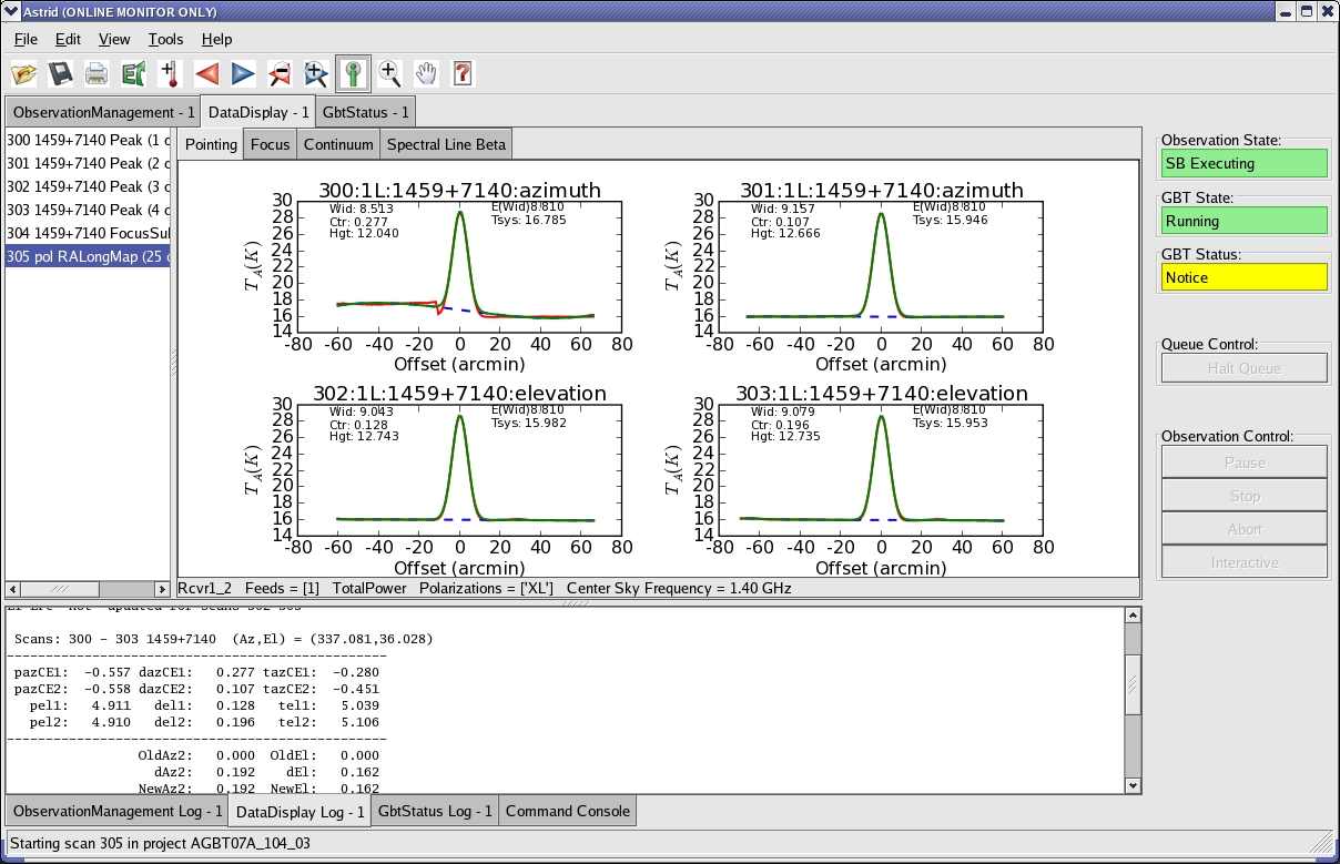
The measured FWHM width (Wid) is shown in arcminutes. The fitted center of the Gaussian (Ctr) is pointing offset in arcmin. The measured height of the Gaussian (Hgt) is in units of the calibrated temperature scale or raw counts (as given by the y-axis label).

The focus scan data will appear under the Focus Tab.

Again, in online mode the data will be processed automatically. They will be calibrated, have a baseline removed and a Gaussian will be fit to the data. The focus offset will automatically be sent to the M&C system.

The details of pointing and focus observations are described in Utility Scan Types.

Fitting Acceptance Options

GFM has several levels of determining whether or not the pointing and focus solutions will be updated in the M&C system. The expected FWHM of the Gaussian fitted to the observed pointing data as the GBT slews across the source should be \(\sim748/\nu_{\text{GHz}}\) arcsec, where \(\nu_{\text{GHz}}\) is the observing frequency in GHz.

For a focus scan the resulting data should approximate a Gaussian with a FWHM of \(1080 \nu_{\text{GHz}}\), in mm. The default behavior for observations below 27 GHz is to assume that a pointing fit is bad if the FWHM differ from the expected value by more than 30% or if the pointing correction is more than twice the FWHM in magnitude; for observations above 27 GHz, the fit is bad if the FWHM differ from the expected value by more than 50% or if the pointing correction is more than three times the FWHM in magnitude. The default for a bad focus scan is if the FWHM is more than 30% from the expected value.

You may change fitting acceptance criteria by:

1. Select the Pointing or Focus Subtab in the DataDisplay tab.

2. Select Tools \(\rightarrow\) Options... from the drop-down menu.

3. Select the new mode in the Fitting Acceptance Criteria tab of the pop-up window.

   Note

   This Option must be set independently for both Pointing and Focus before each type of observation in order to take effect.

The GFM recognizes the fitting acceptance criteria shown below only when AstrID is in one of its online modes.

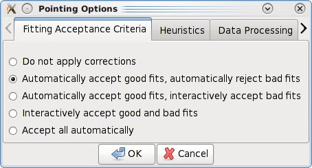
The default setting is to Automatically accept good fits, automatically reject bad fits. You may also choose to never apply corrections or interactively accept bad and/or good fits. There is also an option to Accept all automatically which can be very dangerous and should only be used by experts.

Data Processing Options

You may change the data processing strategy, beams, and/or polarizations used by GFM in reducing pointing or focus scans. This is not needed typically since the software picks the proper default settings under normal conditions. However, for example, if the X polarization channel is faulty for some reason, one can use the Y channel instead. This can be done by:

1. Select the Pointing or Focus Subtab in the DataDisplay tab.

2. Select Tools \(\rightarrow\) Options... from the drop-down menu.

3. Make new data processing selections in the Data Processing Tab of the pop–up window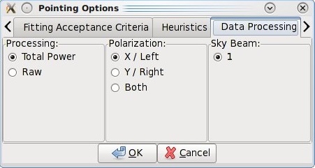

   

   Note

   Options must be set independently for both Pointing and Focus before each type of observation in order to take effect.

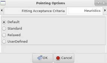
Heuristics Options

Heuristics is a generic term used at the GBT to quantify the “goodness of fit” of the pointing and focus data reduction solutions. Based on the known properties of the GBT, parts of the solution, such as the beamwidth in pointing data, should have certain values within measurement errors. The Heuristics define how large these errors can be. You may change the Heuristics by:

1. Select the Pointing or Focus Subtab in the DataDisplay tab.

2. Select Tools \(\rightarrow\) Options... from the drop-down menu.

3. Select the new mode in the Heuristics tab of the pop-up window

   

   Note

   Options must be set independently for both Pointing and Focus before each type of observation in order to take effect.

The GFM allows you to switch between default, standard, relaxed, and user-defined heuristics. The meaning of standard and relaxed heuristic values are predefined and cannot be changed by you. The standard heuristic expects that the fitted Gaussians have a FWHM within 30% of the expected values and that the pointing solution is within twice the FWHM of the nominal location of the source. For the relaxed heuristics this becomes within 50% of the expected FWHM of the Gaussian fits and three times the FWHM for the pointing correction.

The default option is the software default, and at low frequency (<27 GHz) it is equivalent to standard heurisitics, while at high frequency (>27 GHz) the default mode corresponds to relaxed heursitics. Under normal observing conditions, you should expect to use the default values. Under marginal weather conditions relaxed heuristics may be appropriate even at low frequencies (below 27 GHz). The user-defined heuristic values should only be used by experts. If you wish to use user-defined heuristics then you should contact your GBT project friend.

Sending Corrections

For most observations, GFM processing produces good fits, and the solutions are automatically sent to the telescope using the default settings. However, at high frequencies (especially for W-Band and Argus), fits may fail, and you may want to manually send the corrections to the telescope. You may tell the operator to enter a solution, or you can send the corrections yourself using the Send Corrections functionality.

Note

Corrections show up instantly within the CLEO status window (see XXX), but do not take effect until the start of the next scan.

This can be done by:

1. Select the Pointing or Focus Subtab in the DataDisplay tab.

2. Select Tools \(\rightarrow\) Options... from the drop-down menu.

3. Select the Send Corrections Tab in the pop-up window (if not visible use the arrow button on the right, the Send Corrections tab is farthest to the right)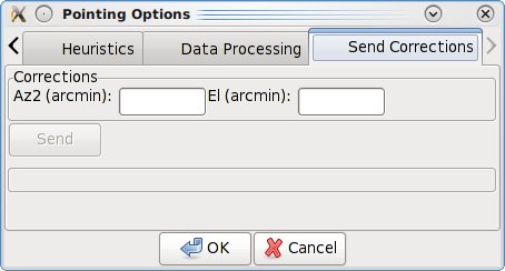

   

4. Enter the corrections in the text box, and click Send to send the solutions to the telescope.

OOF Data Display

Out-of-focus holography (OOF) is a technique for measuring large-scale errors in the shape of the reflecting surface by mapping a strong point source both in and out of focus. The procedure derives surface corrections which can be sent to the active surface controller to correct surface errors. The procedure is only recommended for observing at frequencies of 40 GHz and higher.

The AutoOOF() procedure will obtain three OTF maps, each taken at a different focus position. Processing will begin automatically upon completion of the third map, the status of which can be viewed in the progress bar under AutoOOF Processing Status on the right-hand-side of the screen. Once complete, the result will be displayed in the OOF subtab of the AstrID DataDisplay.

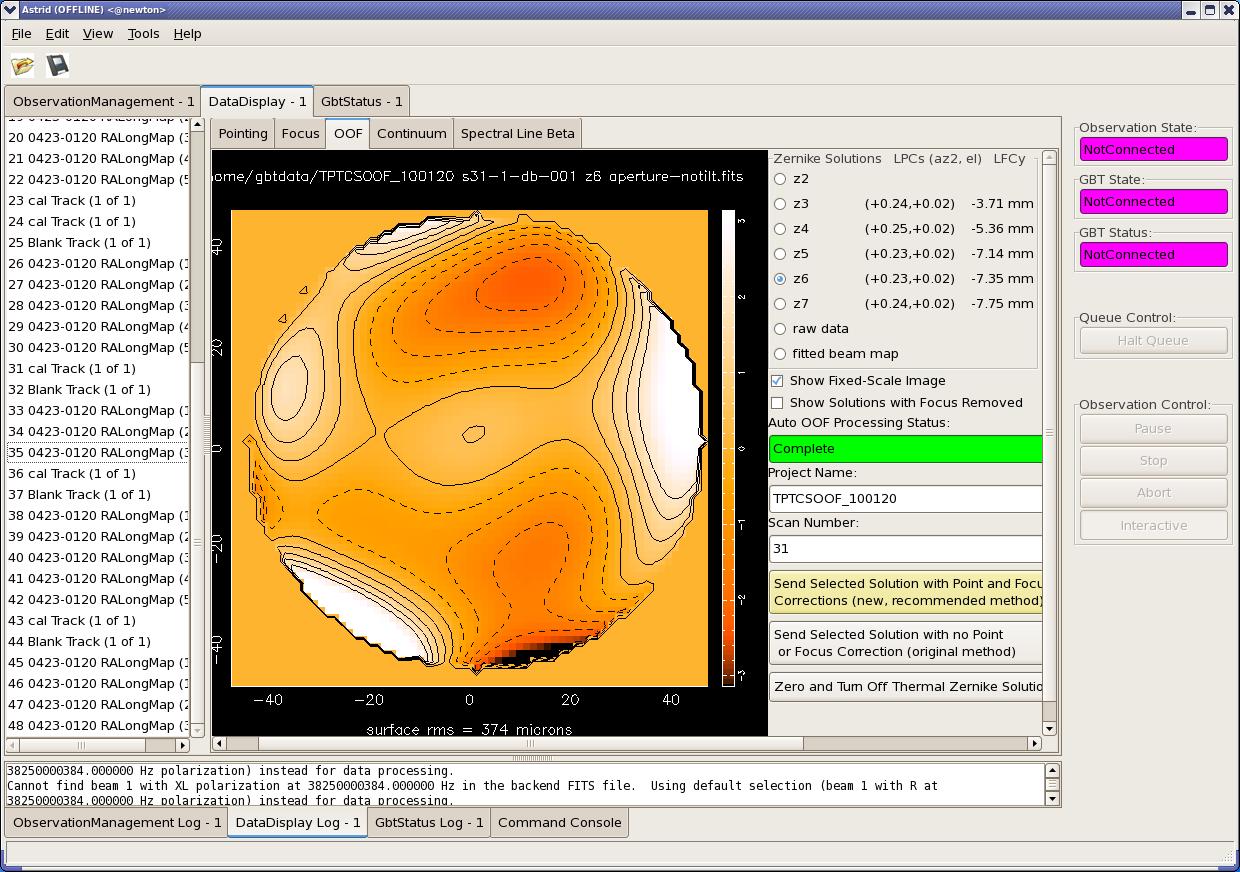
Once processing is complete, the default solution displayed in AstrID is the fifth-order Zernike fit (z5). The most aggressive fit is z6, while z3 is less aggressive. Solutions may be selected and viewed via the radio buttons in the upper-right section of the screen. Derived Local Pointing Corrections (LPCs) in arcminutes, and Local Focus Corrections (LFCy) in millimeters are displayed to the right of each radio button. Raw AutoOOF data at each focus position can be viewed as a timestream and map by selecting the raw data radio button. The fitted beam map radio button will display fitted beam map images and reduced \(\chi^{2}\) values for the three highest orders of Zernike fits (z3, z4, and z5 by default).

Solutions must be chosen by the observer and manually sent to the active surface. Therefore, it is essential that the Zernike fits and raw AutoOOF data are examined carefully before deciding upon a solution. Steps for validating and discerning appropriate solutions can be found in AutoOOF Guide.

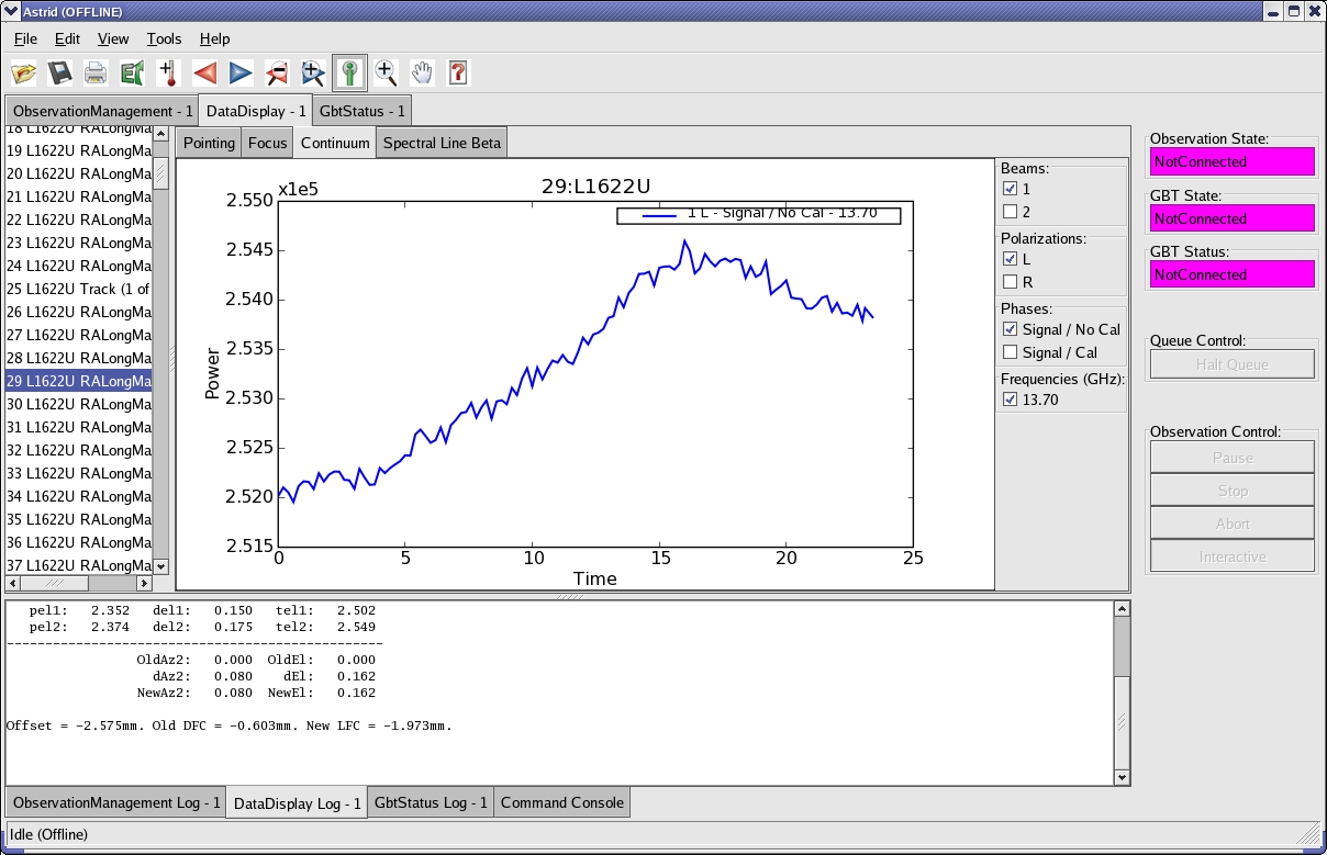
Continuum Data Display

Continuum data taken with the GBT that are not part of pointing and focus scans will show up in plots under the Continuum Tab. This will show the uncalibrated continuum data as a function of time only.

Spectral Data Display

The Spectral Line Display was a tool originally designed for browsing the previous GBT Spectrometer spectral line data.

When viewing data online, the most recent integration is plotted automatically. Individual integrations may be selected and viewed offline. Here is an example of the spectral line data display.

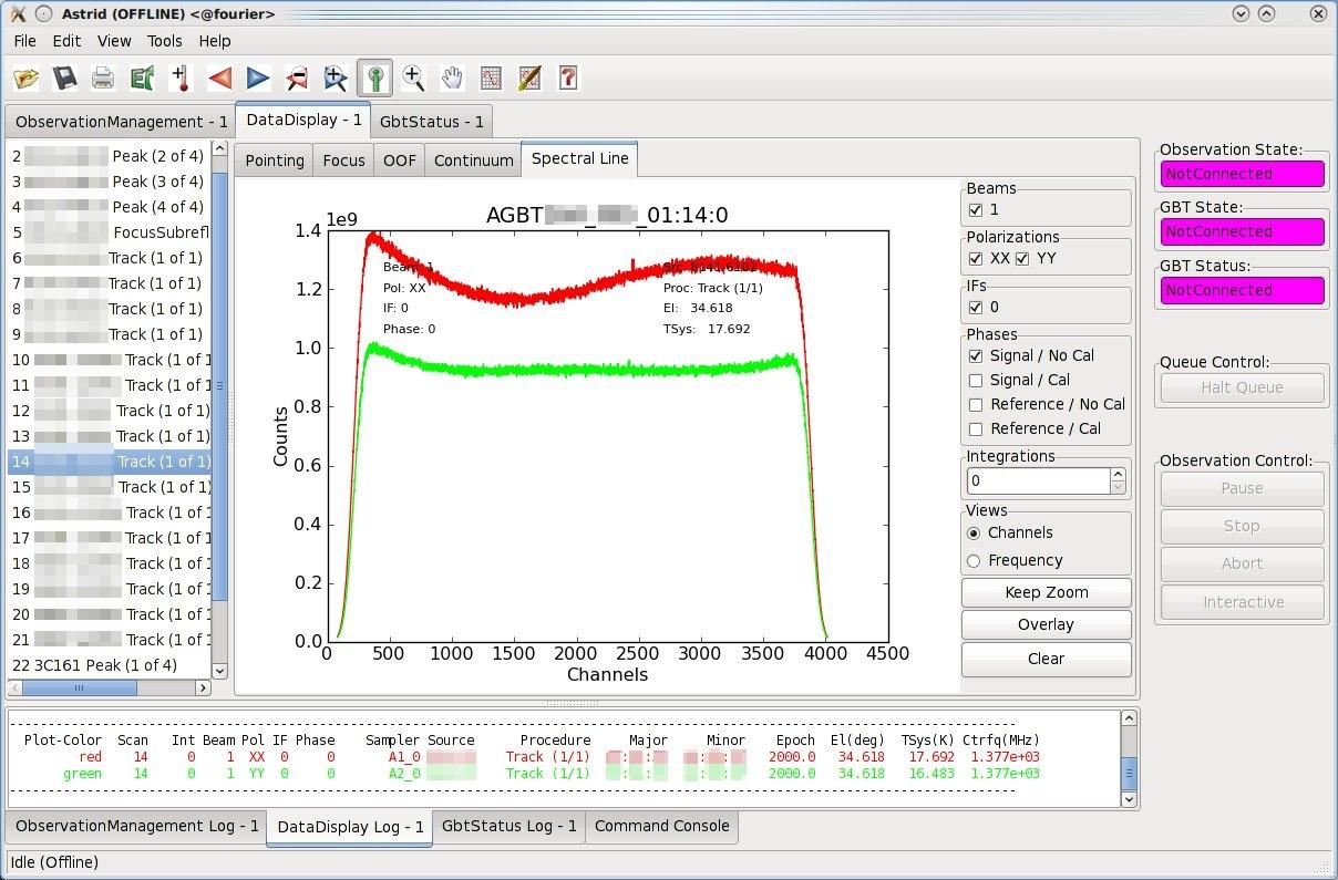
The spectra displayed are raw data and no calibration has been applied to them. As spectra are plotted, information about each plot is printed in the console window. Each line is color coded to match the color of that spectrum in the plotting window. In addition, some of the information for the very first spectra are used to annotate the plot. The plot title is parsed as project_name:scan_number:integration_number. For offline usage, the desired integration can be selected either using the up/down arrows, or by typing in a value in the edit box.

All user interaction for this plugin occurs in the right-hand side options panel. The check boxes allow selection of spectra to plot via astronomical variables: Beams, Polarizations, IF numbers, and Phases. The options panel also includes three buttons and a radio box for plot viewing. The Views radio box offers options for plotting the bandpass vs. Channels or Sky Frequency. The Keep Zoom toggle button will maintain the current zoom, even as new spectra are plotted. Using the unzoom command (mouse right-click, or via the toolbar) will return the plot to its original scale. The Overlay toggle button can be used to overplot spectra from different integrations or scans. Finally, the Clear button erases the plot.

Data Display Plotting Panel Toolbar

The plotting panel toolbar allows user interactions with plots in the display window and is located near the top of the Astrid Screen. The following features are available:

	Open	Allows the user to open a previously saved session. This has the same functionality as File \(\rightarrow\) Open... described in Working Offline.
	Save	Allows the user to save output from the data display log as a text file.
	Print	DO NOT USE, Please use the Export function instead.
	Export	Allows the user to save the figure displayed in the plotting panel to a file. The name must have an extension of either .png, .ps or .eps.
	Unfreeze	Not applicable to Astrid general use. Unfreezes the processing of commands via the command line and intended for use in conjunction with the Freeze command.
	Undo	Undoes your last command.
	Redo	Redoes your last command.
	Unzoom	Undoes a previously executed zoom.
	Rezoom	Redoes a previously executed zoom.
	Info Tool	Selecting the info tool allows the user to use the mouse pointer to focus in/out among the available subplots (e.g., peak scans). Left-clicking the mouse brings a subplot into focus (hiding the other subplots). Right-clicking the mouse on the focused plot will show all subplots. If there is only one subplot, the info tool simply displays the mouse xy coordinates.
	Zoom Tool	Selecting the zoom tool allows the user to use the mouse pointer for zooming in on a particular area of the plot. Left-clicking the mouse will zoom in. Right-clicking the mouse will zoom out.
	Pan Tool	Allows the user to use the mouse pointer to pan around the selected subplot. Left-clicking the mouse and holding the left button down will pan around the subplot. Right-clicking restores the original view.
	Grid Tool	Turns on the plot grid.
	Plot Edit Tool	Allows you to edit plot labels, colors, and title. Clicking on “Advanced Options” brings up an additional dialog which contains options for transparency, legend placement, and ordering of plots. Colors may be entered as hex codes or selected by clicking on the colored button to the right of the text field. Plots can only be reordered within their subplot - i.e., Y1 lines will always be below Y2 lines. Legend location can be specified with simple strings (e.g., “upper right”) or coordinates 0-1 along the plot edges. If a string is chosen it will be used in place of any coordinates.
	User Manual	Displays the Data Extraction and Analysis Program (DEAP) user manual.

Todo

Transfer DEAP user manual to GBTdocs.

Use of Plotting Capabilities

A User Manual is available http://deap.sourceforge.net/help/index.html that describes all the plotting functionality available in GFM. There is also a plotting Tutorial that illustrates the plotting capabilities by example which is available at http://deap.sourceforge.net/tutorial/index.html.

Todo

Transfer the guide and tutorial to GBTdocs.

GbtStatus Tab

The GbtStatus Tab displays various GBT specific parameters, sampled values and computed values. Special care was taken to promote its use for remote observing. An Example of how the GBT Status Display appears in AstrID is shown in Figure~ref{fig:astridstatusone} and~ref{fig:astridstatustwo}.

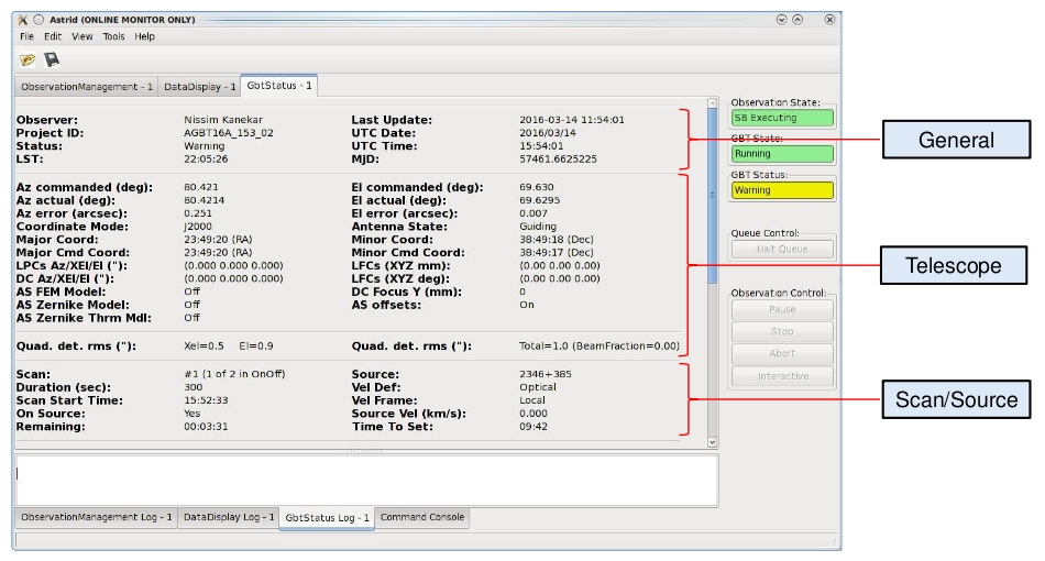
Fig. 25 The top portion of the AstrID GbtStatus Tab. To see the rest of the status screen you will need to use the scroll bar.

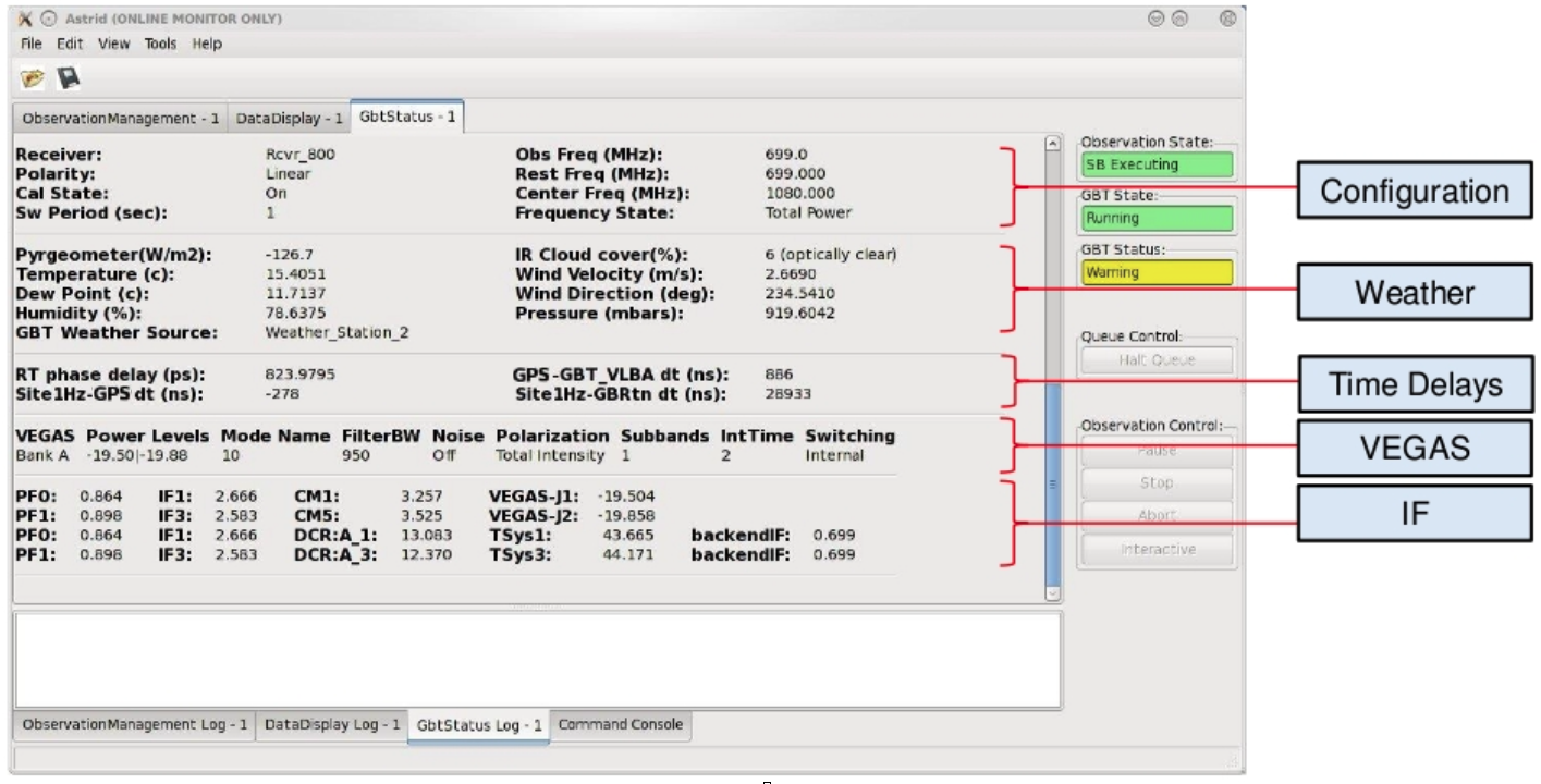
Fig. 26 The bottom portion of the AstrID GbtStatus Tab. To see the rest of the status screen you will need to use the scroll bar.

General Status

Observer	The observer name
Project ID	The data directory of the FITS files. This is your Project Name with the session as a suffix. For example, the Project ID for session 02 of AGBT16A_001 would be AGBT16A_001_02. See Project Name and List of SBs for details.
Status	The status of the GBT. See State for details.
LST	The Local Sideral Time of the last update
Last Update	The local time when the database was last updated
UTC Date	The Coordinated Universal Time date of the last update
UTC Time	The Coordinated Universal Time time of the last update
MJD	The Modified Julian Date of the last update

Telescope Status

Az commanded	The commanded azimuth position of the telescope in degrees.
Az actual	The actual azimuth position of the telescope in degrees.
Az error	The difference between the commanded and the actual azimuth position of the telescope in arc-seconds. This value does not contain a \(\cos\left({\text{el}}\right)\) correction
El commanded	The commanded elevation position of the telescope in degrees.
El actual	The actual elevation position of the telescope in degrees.
El error	The difference between the commanded and the actual elevation position of the telescope in arc-seconds.
Coordinate Mode	The coordinate mode used to represent a particular location on the sky. See Location object for more information.
Major and Minor Coord	The telescope position in the current Coordinate Mode.
Major and Minor Cmd Coord	The telescope position in the current commanded Coordinate Mode.
Antenna State	Disconnected - antenna software is not running Dormant - antenna software is running but with its control of the antenna turned off Stopped- antenna is not moving Guiding- antenna is moving and data are being taken Tracking- data are not being taken Slewing - antenna is moving to a new commanded position
LPCs Az/XEl/El	The Local Pointing Correction (LPC) offsets in arc-seconds.
DC Az/XEl/El	The DC values in arc-seconds. The GBT has temperature sensors attached at various points on the backup structure and the feed-arm. These are used in a dynamic model for how the GBT flexes with changing temperatures. This model is used to correct for pointing and focus changes that occur from this flexing.
LFCs (XYZ mm)	The Local Focus Correction (LFC) for the offset focus position in millimeters. This value is determined from a Focus observation
LFCs (XYZ deg)	The subreflector tilt offset in degrees.
DC Focus Y (mm)	The DC Y subreflector offset in millimeters.
AS FEM Model	The state of the Finite-Element Model (FEM) correction for the Active Surface (AS). The FEM predicts how the surface changes due to gravitional flexure versus the elevation angle.
AS Zernike Model	The state of the AS Zernike model correction model. The Zernike model is a set of Zernike polynomial coefficients determined from Out-Of-Focus (OOF) holography that improve the shape of the AS versus the elevation angle.
AS Zernike Thrm Model	The state of the FEM correction for the AS. The FEM predicts how the surface changes due to thermal flexure.
AS Offsets	The state of the AS zero offsets. The zero offsets are the default positions for the AS. This should always be On if the AS is being used.
Quad. det. rms	The quadrant detector is used to detect and correct for wind-induced pointing errors. rms values in arc-seconds are reported in elevation and cross-elevation. Total rms is also given as a fraction of the beam.

Scan and Source Status

Scan	A scan is a command within an SB used to collect observational data. The field here is derived from the scan number and PROCNAME, PROCSIZE and ``PROCSEQN keywords from the GO FITS file.
Duration	The scan length in seconds.
Scan Start Time	If scan has started it is the UTC scan start time - if the scan has not started, then it is the countdown until the start of scan.
On Source	Yes or displays a countdown until the antenna is on source.
Remaining	The time remaining in the scan.
Source	The source name.
Vel Def	The velocity definition specifies which mathematical equation is used to convert between frequency and velocity. Todo Add reference to Explanation section (TBW)
Vel Frame	The velocity frame or inertial reference frame. See vframe (str) for more information.
Source Vel	The source velocity (km \({\text{s}}^{-1}\)).
Time To Set	The time till the current source sets.

Configuration Status

Receiver	The receiver being used.
Polarity	The receiver polarity.
Cal State	ON if the noise diode is firing during the scan
Sw Period	The period in seconds over which the full switching cycle occurs. This is determined by the user in their configuration. See swper (float) for more information.
Obs Freq	The observed spectral line frequency in the local frame (MHz).
Rest Freq	The spectral line frequency in the rest frame (MHz).
Center Freq	The center IF frequency set by the LO in MHz. See here for further details
Frequency State	The switching type. Either “total power” or “frequency-switching”.

Weather Status

A real–time readout from one of the gls{GBT} weather stations providing information on temperature, pressure, humidity, dew point, wind direction and velocity. In addition, the pyrgeometer measures the net near-IR irradiance of the sky to give an approximate indication of cloud cover.

Note

The pyrgeometer is currently not active.

Time Delay Status

RT phase delay	This is the time delay between the timing center in the GBT equipment room and the GBT receiver room, in picoseconds, modulo 2000 ps. It is measured by comparing the phase of the 500 MHz reference signal sent to the receiver room with a copy of the signal returned to the timing center.
Site1Hz-GPS dt	Time difference between the Site1Hz (a one pulse per second signal that is locked to the hydrogen maser time standard) and a pulse from the GPS receiver.
GPS-GBT_VLBA dt	Time difference between the GPS receiver and the VLBA backend timing module.
Site1Hz-GBTRtn dt	Time delay between the Site 1Hz and a copy of the 1 Hz returned from GBT receiver room. It is twice the delay of the fiber cables. The value is about 28933 ns which means the time delay between the equipment room the the receiver room is about 14466 ns.

VEGAS Status

VEGAS	The VEGAS Bank (spectrometer with letter designation A \(\rightarrow\) H) selected in the scan coordinator.
Power Levels	The power levels at the inputs to the VEGAS ADC cards. There are two ADCs per bank, one for each polarization. The VEGAS balance API sets these values to approximately -20dBm by default.
Mode Name	Each VEGAS Bank can be configured in 1 of 29 Spectral Modes (Table 15) or 1 of 24 Pulsar Modes (Table 18 and Table 19).
FilterBW	The bandwidth (MHz) of the digital filter implemented in the FPGA. Note These values do not correspond to the bandwidths listed in Table 15.
Noise	The state of the noise source which can be either On or Off.
Polarization	Users may specify which spectral product to record (see vegas.vpol (str) for more information).
Subbands	Each VEGAS bank can select between single (subbands=1) and multiple (subbands=8) spectral windows when using VEGAS modes with a 23.44 MHz bandwidth.
IntTime	The VEGAS integration (dump) time in seconds.
Switching	Determines whether switching is controlled by VEGAS (“Internal”) or another source (“External”).

IF Status

The IF path in use is always displayed in the last section of the GBT status screen. An example screen is shown in Figure The bottom portion of the AstrID GbtStatus Tab. To see the rest of the status screen you will need to use the scroll bar.; the content displayed depends on the exact configuration. In this example, each line represents the IF path for a single polarization path from the IF rack to the backend. Each line contains only the devices in use for the listed path. A path may include a subset of the devices and values listed below.

IF#	The # displayed is the number corresponding to the IF rack switch in use. The value displayed is the RF power in Volts detected by the IF rack.
CM#	The # displayed is the number corresponding to the Converter Module in use. The value displayed is the RF power in Volts coming out of the Converter Module after the LO2 and LO3 mixers and before the Converter Module filters.
CF#	The # displayed is the number corresponding to the Analog Filter in use. The value displayed is the RF power in Volts coming out of the AF rack after all filters have been applied (used with 100 MHz converters).
SG#	The # displayed is the number corresponding to the Analog Filter in use. The value displayed is the RF power in Volts coming out of the AF rack after all filters have been applied (used with 1.6 GHz samplers).
VEGAS-J#	The # displayed is the number corresponding to the port of VEGAS0 in use. The value displayed is the power level in dBFS. For best performance, it should be approximately -20 dBFS.
Radar-Port#	The # displayed is the number corresponding to the port of the Radar in use.
DCR:A_#	The # displayed is the bank and number corresponding to the port of the DCR in use. The value displayed is the total power in raw counts.
TSys#	The # displayed is the number corresponding DCR port in use. The value displayed is the system temperature as reported by the DCR (should be considered a loose approximation).
backendIF	The value displayed is the frequency of the Doppler track rest frequency as seen by the backend, in GHz.