CCB

CCB#

The CCB is a sensitive, wideband backend designed exclusively for use with the GBT Ka-band receiver, build in collaboration with A.C.S. Readhead’s radio astronomy instrumentaiton group at Caltech, It was commissioned on the GBT in 2006.

The driving consideration behind its design is to provide fast electronic beam switching in order to suppress the electronic gain fluctuations which usually limit the sensitivity of continuum measurements with single dish radio receivers. To further improve stability, it is a direct detection system: there are no mixers before the conversion from RF to detected power. The Ka-band receiver provides eight simultaneous, directly detected channels of RF power levels to the CCB: one for each feed, times four frequency channels (26-29.5 GHz; 29.5-33 GHz; 33-36.5 GHz; and 36.5-40 GHz). Astronomical information and labels for these 8 channels (or ports in GBT parlance) are summarized below:

Table 21 CCB port labels and the astronomical quantities they measure#
Port	Beam	Polarization	Frequency
9	1	Y	38.25
10	1	Y	34.75
11	1	Y	31.25
12	1	Y	27.75
13	2	X	38.25
14	2	X	34.75
15	2	X	31.25
16	2	X	27.75

It provides carefully optimized radio frequency (not an intermediate frequency) detector circuits and the capability to beam-switch the receiver rapidly to suppress instrumental gain fluctuations. There are 16 input ports (only 8 can be used at present with the Ka-band receiver), hard-wired to the receiver’s 2 feeds x 2 polarizations x 4 frequency sub-bands. The CCB allows the left and right noise-diodes to be controlled individually to allow for differential or total power calibration. Unlike other GBT backends, the noise-diodes are either on or off for an entire integration (there is no concept of phase within an integration). The minimum practical integration period is 5 milliseconds; integration periods longer than 0.1 seconds are not recommended. The maximum practical beam-switching rate is about 4 kHz, limited by the needed \(250\mu s\) beam-switch blanking time. Switching slower than 1 kHz is not recommended.

The following sections outline the process of observing with, and analyzing the data from, the CCB.

Much of the information in this chapter is also maintained at /users/bmason/ccbPub/README.txt.

Todo

Move Brian’s CCB part entirely to GBTdocs.

Observing with the CCB#

Configuration#

Configuration of the CCB is straightforward, and for most purposes the only two configurations are needed:

ccb.conf - integration time of 4 milliseconds, useful for estimating the scatter in the samples to obtain meaningful \(\chi^2\) values in the analysis of science data
ccbbothcalslong.conf - integration time of 25 miliseconds, useful in preak/focus observations to speed up processing of the data.

ccb.conf

# tell AstrID to expect beam-switched continuum observations
# with Ka-band and the CCB
# note: These keywords do not have any practical effect on
#       the actual instrument configuration but they are 
#       necessary to set up internal variables and ensure 
#       the recorded fits files are accurate.
   
receiver    = 'Rcvr26_40'
beam        = 'B12'
obstype     = 'Continuum'
backend     = 'CCB'
nwin        = 4
restfreq    = 27000, 32000, 35000, 38000
deltafreq   = 0, 0, 0, 0
bandwidth   = 600, 600, 600, 600
swmode      = 'sp'
swtype      = 'bsw'
pol         = 'Circular'
vdef        = 'Radio'
vframe      = 'topo'

# integration time in seconds

tint        = 0.005

# backend specific keywords
#   specify the cal firing pattern

ccb.cal_off_integs  = 20
ccb.XL_on_integs    = 2
ccb.both_on_integs  = 2
ccb.YR_on_integs    = 2

#   specify the beam switching frequency in kHz
#   note: setting this value to 4 causes a 
#         ">10% blanking" warning, which may
#         be safely ignored

ccb.bswfreq         = 4

ccbbothcalslong.conf

# tell AstrID to expect beam-switched continuum observations
# with Ka-band and the CCB
# note: These keywords do not have any practical effect on
#       the actual instrument configuration but they are 
#       necessary to set up internal variables and ensure 
#       the recorded fits files are accurate.
   
receiver    = 'Rcvr26_40'
beam        = 'B12'
obstype     = 'Continuum'
backend     = 'CCB'
nwin        = 4
restfreq    = 27000, 32000, 35000, 38000
deltafreq   = 0, 0, 0, 0
bandwidth   = 600, 600, 600, 600
swmode      = 'sp'
swtype      = 'bsw'
pol         = 'Circular'
vdef        = 'Radio'
vframe      = 'topo'

# integration time in seconds

tint        = 0.025

# backend specific keywords
#   specify the cal firing pattern

ccb.cal_off_integs  = 20
ccb.XL_on_integs    = 2
ccb.both_on_integs  = 2
ccb.YR_on_integs    = 2

#   specify the beam switching frequency in kHz
#   note: setting this value to 4 causes a 
#         ">10% blanking" warning, which may
#         be safely ignored

ccb.bswfreq         = 4

Pointing & Focus#

The online processing of pointing and focus data is handled by GFM (which runs within the AstrID Data Display window) similarly as for other GBT receivers and the DCR. A few comments:

Because the Kaband receiver currently only has one polarization per beam, GFM will by default issue some complaints which can be ignored. These can be eliminated by choosing Y/Right polarization in the AstrID Data Display window under Tools \(\rightarrow\) Options \(\rightarrow\) Data Processing.
In the same menu (Tools \(\rightarrow\) Options \(\rightarrow\) Data Processing), choosing 31.25 GHz as the frequency to process, instead of the default 38.25 GHz, can improve robustness of the result.
The results shown in the AstrID Display are in raw counts, not Kelvin or Janskys.
Processing the data with Relaxed heuristics is also often helpful, which is the default processing option for Ka-band

There is a template pointing and focus SB for the CCB in /users/bmason/ccbPub called ccbPeak.turtle (see below). This scheduling block does a focus scan, four peak scans, and a symmetric nod (for accurate photometry to monitor the telescope gain).

########################################################
#
# 31jan06 bsm -- SB for peak/focus checks with CCB
#                          Also does a nod on the calibrator source.
#
########################################################

#######################################################
# 
# configuration variables
#  

# your source should be in the default gbt pointing catalog
#  which is at /home/astro-util/pointing/pcals4.0/pntKaband.cat
mySrc= "0241-0815"

Catalog()

#
# You shouldn't have to change anything below here
#
#######################################################

Slew(mySrc)                                        
Configure("/users/bmason/ccbPub/ccbbothcalslong.conf")			       
execfile("/users/bmason/ccbPub/addwx.py")
execfile("/users/bmason/ccbPub/killlo.py")			       
execfile("/users/bmason/ccbPub/deselectDeadCcbChans.py")			       
AutoPeakFocus(source=mySrc,configure=False)

trajdir="/users/bmason/gbt-dev/scanning/ptcsTraj"
if (trajdir not in sys.path):
	sys.path.append(trajdir)
from readFitsTraj import readFitsTraj

#
# Read in the trajectories
#
trajnod=readFitsTraj("/users/bmason/ccbPub/ka-otfnod-symmShort.fits",1.0)
DefineScan("dotrajectory", "/users/bmason/gbt-dev/scanning/ptcsTraj/dotrajectory.py")

Configure("/users/bmason/ccbPub/ccb.conf")
execfile("/users/bmason/ccbPub/addwx.py")
execfile("/users/bmason/ccbPub/killlo.py")
execfile("/users/bmason/ccbPub/deselectDeadCcbChans.py")			       
Slew(mySrc)
dotrajectory(trajnod,location=mySrc, beamName="1", cos_v=True,  coordMode="Encoder") 

Observing Modes & Scheduling Blocks#

Science projects with the CCB typically fall into two categories: mapping, and point source photometry. The majority of CCB science is the latter, since this is what, by design, it does best. Template scheduling blocks for both are in /users/bmason/ccbPub.

Todo

Move those templates here.

Note

We strongly encouraged you to use these template scheduling blocks as the basis for your CCB observing scripts and make only the changes that are required! Relatively innocuous changes can make the data difficult or impossible to calibrate with existing analysis software.

The basic template SB are:

ccbObsCycle.turtle: perform photometry on a list of sources.
ccbRaLongMap.turtle: perform a standard RALongMap() on a source.
ccbMap.turtle, ccbMosaicMap.turtle: make maps using longer, single-scan, custom raster maps. Your project friend will help tailor these to your project’s needs, should you choose this approach.

ccbObsCycle.turtle

########################################################
#
# 26jan06
#  template scheduling block for GBT CCB observations
#
# Uses new symmetric otf nods with 10 sec per phase and
#  10 sec initial settle
#
#  This scan takes 1.5m per source including intrasource slew
#  During the day you should have 20 sources in this block plus
#   the peak/focus
#  During the night you can let it slip to 27 sources plus
#   peak/focus
#  Take care that if you increase the value of NNODS below
#   (the number of nods done on  each source) to decrease
#   the number of sources commensurately.
#
########################################################

#######################################################
# 
# configuration variables
#  
#######################################################

# number of nods to do on each source
nnods=1

#
# sources to observe in this scheduling block.
#
srclist=[
"020003+0013",
"020056+0004",
"020108+0009",
"015859+0013",
"020145+0007",
"015842+0024",
"015802+0018",
"020048+0034",
"020056+0033",
"020053+0025"]


# the above sources must be in this
# ASTRID format catalog:
targetcat=Catalog("/users/bmason/ccbPub/example.acat")

#
# NB: which catalog you gotta be in is defined by the "isCal" fields
#  in the above array
#
########################################################
# You shouldn't have to change anything below this line
#
#######################################################

###############################################
#
# Define custom scan "dotrajectory" 
#  also define the function that reads in a trajectory FITS file,
#  and then use it, to read in some trajectories.
#

import os
import sys

trajdir="/users/bmason/gbt-dev/scanning/ptcsTraj"
if (trajdir not in sys.path):
	sys.path.append(trajdir)
from readFitsTraj import readFitsTraj

#
# Read in the trajectories
#
trajnod=readFitsTraj("/users/bmason/ccbPub/ka-otfnod-symmShort.fits",1.0)
DefineScan("dotrajectory", "/users/bmason/gbt-dev/scanning/ptcsTraj/dotrajectory.py")

# set an initial configuration and add the weather data to the archivist
#  if the first source is not a calibrator this also leaves us in a
#  happy state for CCB observations
Configure("/users/bmason/ccbPub/ccb.conf")
execfile("/users/bmason/ccbPub/addwx.py")
execfile("/users/bmason/ccbPub/killlo.py")
execfile("/users/bmason/ccbPub/deselectDeadCcbChans.py")			       

srccnt=0
for mySrc in srclist:
   SetValues("ScanCoordinator", {"source": mySrc} )
   Slew(mySrc)
   for iter in xrange(nnods):
      dotrajectory(trajnod,location=mySrc, beamName="1", cos_v=True,  coordMode="Encoder")


Comment("END OF SCHEDULING BLOCK")

ccbRALongMap.turtle

ccbMap.turtle

########################################################
#
#  19apr07 ccb mapping SB
#          Uses trajectory in independent fits file
#
#  With default file kaRaster5x2-6sec does a 5'x2' square
#   map in just over 4 minutes.
#
#  You can also just use standard RALongMap instead of 
#   the single trajectory, though this is 
#   less efficient and may excite more feedarm 
#   vibration.
#
########################################################


# the above sources must be in this
# ASTRID format catalog:
targetcat=Catalog("/users/bmason/ccbPub/example.acat")
# or in the default catalog...
Catalog()

mySrc="0241-0815"

###############################################
#
# Define custom scan "dotrajectory" 
#  also define the function that reads in a trajectory FITS file,
#  and then use it, to read in some trajectories.
#

import os
import sys

trajdir="/users/bmason/gbt-dev/scanning/ptcsTraj"
if (trajdir not in sys.path):
	sys.path.append(trajdir)
from readFitsTraj import readFitsTraj
from offsetFitsTraj import offsetFitsTraj

#
# Read in the trajectory
#
traj=readFitsTraj("/users/bmason/ccbPub/karaster5x2-6sec.fits",1.0)
DefineScan("dotrajectory", "/users/bmason/gbt-dev/scanning/ptcsTraj/dotrajectory.py")

# set an initial configuration and add the weather data to the archivist
#  if the first source is not a calibrator this also leaves us in a
#  happy state for CCB observations
Configure("/users/bmason/ccbPub/ccb.conf")
execfile("/users/bmason/ccbPub/addwx.py")
execfile("/users/bmason/ccbPub/killlo.py")
execfile("/users/bmason/ccbPub/deselectDeadCcbChans.py")			       

Slew(mySrc)
dotrajectory(traj,location=mySrc, beamName="1", cos_v=True,  coordMode="Encoder")

# offset by 2 arcmin in the vertical direction (in whatever coordinate system
#  the offset is being applied -- here Encoder ie az/el)
traj=readFitsTraj("/users/bmason/ccbPub/karaster5x2-6sec.fits",1.0)
offsetFitsTraj(traj,0.0,2.0/60.0)
dotrajectory(traj,location=mySrc, beamName="1", cos_v=True,  coordMode="Encoder")

# offset by 4 arcmin in the vertical direction (in whatever coordinate system
#  the offset is being applied -- here Encoder ie az/el)
traj=readFitsTraj("/users/bmason/ccbPub/karaster5x2-6sec.fits",1.0)
offsetFitsTraj(traj,0.0,4.0/60.0)
dotrajectory(traj,location=mySrc, beamName="1", cos_v=True,  coordMode="Encoder")

ccbMosaicMap.turtle

########################################################
#
#  19apr07 ccb mapping SB
#          Uses trajectory in independent fits file
#
#  With default file kaRaster15x2-6sec does a 15'x2' square
#   map in ~5.4 minutes.
#  Repeat this 5 times, with centers spaced by 1'52", to
#   build up a 15'x10' map
#
#  You can also just use standard RALongMap instead of 
#   the single trajectory, though this is 
#   less efficient and may excite more feedarm 
#   vibration.
#
########################################################


# the above sources must be in this
# ASTRID format catalog:
targetcat=Catalog("/users/bmason/ccbPub/example.acat")
# or in the default catalog...
Catalog() 

sourcelist=[
"ldn1622n2",
"ldn1622n1",
"ldn1622",
"ldn1622s1",
"ldn1622s2"]

###############################################
#
# Define custom scan "dotrajectory" 
#  also define the function that reads in a trajectory FITS file,
#  and then use it, to read in some trajectories.
#

import os
import sys

trajdir="/users/bmason/gbt-dev/scanning/ptcsTraj"
if (trajdir not in sys.path):
	sys.path.append(trajdir)
from readFitsTraj import readFitsTraj

#
# Read in the trajectory
#
#trajnod=readFitsTraj("/users/bmason/ccbPub/karaster15x2-6sec.fits",1.0)
trajnod=readFitsTraj("/users/bmason/ccbPub/karaster5x2-6sec.fits",1.0)
DefineScan("dotrajectory", "/users/bmason/gbt-dev/scanning/ptcsTraj/dotrajectory.py")

# set an initial configuration and add the weather data to the archivist
#  if the first source is not a calibrator this also leaves us in a
#  happy state for CCB observations
Configure("/users/bmason/ccbPub/ccb.conf")
execfile("/users/bmason/ccbPub/addwx.py")
execfile("/users/bmason/ccbPub/killlo.py")
execfile("/users/bmason/ccbPub/deselectDeadCcbChans.py")			       

for mysrc in srclist:
   Slew(mySrc)
   dotrajectory(trajnod,location=mySrc, beamName="1", cos_v=True,  coordMode="Encoder")

Point source photometry is accomplished with an OTF variant of the symmetric Nod() procedure. This procedure, which we refer to as the OTF-NOD, alternately places the beam in each of the two beams of the Ka-band receiver in a B1/B2/B2/B1 pattern. This sequence cancels means and gradients in the atmospheric or receiver emission with time. Plotting the beamswitched data from this sequence produces a sawtooth pattern shown in Figure~ref{fig:otfnodconcept}; this is discussed more in S~ref{sec:onlineanalys}.

Each NOD is 70 seconds long (10 seconds in each phase, with a 10 second slew between beams and an initial 10 second acquire time).

Note

OTF-NOD is not one of the standard scan types; it is implemented in the scripts mentioned here (e.g., ccbObsCycle.turtle).

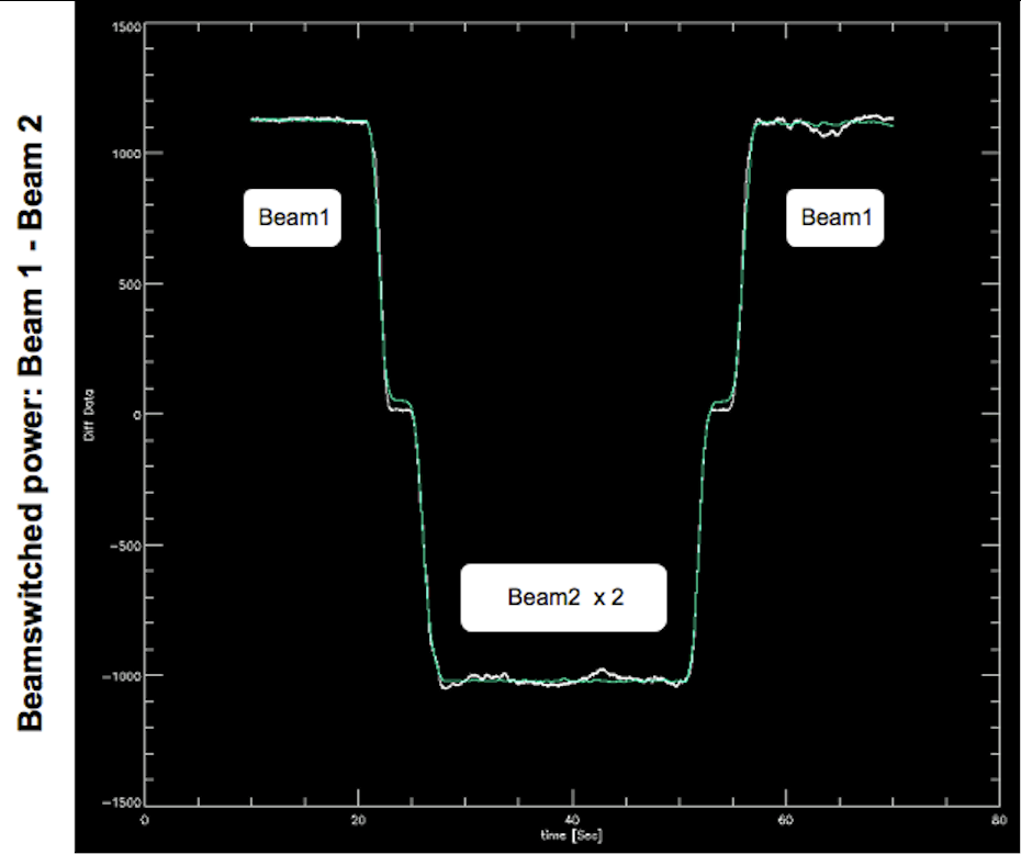
../../_images/ccbTutorial23feb09-010.png — Fig. 50 Data from a CCB, beamswitched OTF-NOD, showing data and model versus time through one B1/B2/B2/B1 scan. The white line is the CCB beam-switched data and the green line is the fit for source amplitude using the known source and telescope (as a function of time) positions.#

Calibration#

If at all possible, be sure to do a peak and focus, and perform photometry (an OTF-NOD, as implemented in ccbObsCycle.turtle or ccbPeak.turtle) on one of the following three primary (flux) calibrators: 3c48, 3c147, or 3c286. This will allow your data to be accurately calibrated (our calibration scale is ultimately referenced to the WMAP 30 GHz measurements of the planets). If this is not possible the calibration can be transferred from another telescope period (observing session) within a few days of the session in question.

Online Data Analysis#

It is important to assess data quality during your observing session. There are a set of custom IDL routines for analyzing CCB data; if you use the observing procedures and config files described here, your data should be readily calibratable and analyzable by them. To use the IDL code, start IDL by typing (from the GB UNIX command line):

/users/bmason/ccbPub/ccbidl

Example OTF-NOD data for bright sources (under good and poor conditions) and a weak source (under good conditions) are shown in Figures~ref{fig:brightgood} through ref{fig:weakbinned}.

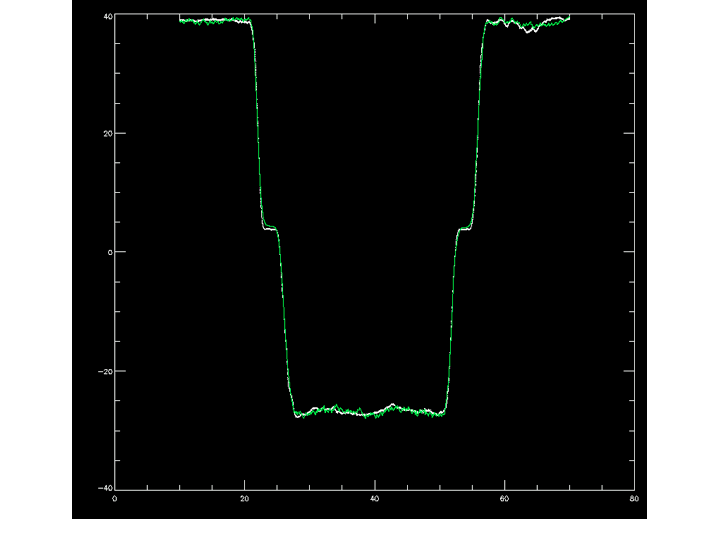
../../_images/ccbTutorial23feb09-011.png — Fig. 51 CCB data from an OTF-NOD observation of a bright source, showing data and model versus time through one B1/B2/B2/B1 scan. The white line is the CCB beam-switched data and the green line is the fit for source amplitude using the known source and telescope (as a function of time) positions. The close agreement between the data and the fit indicate that neither fluctuations in atmospheric emission nor pointing fluctuations (typically due to the wind on these timescales) are problems in this data.#

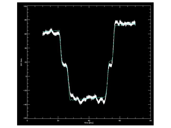
../../_images/ccbTutorial23feb09-012.png — Fig. 52 CCB OTF-NOD data on a bright source under marginal conditions.The differences between the data and the model are clearly larger in this case.#

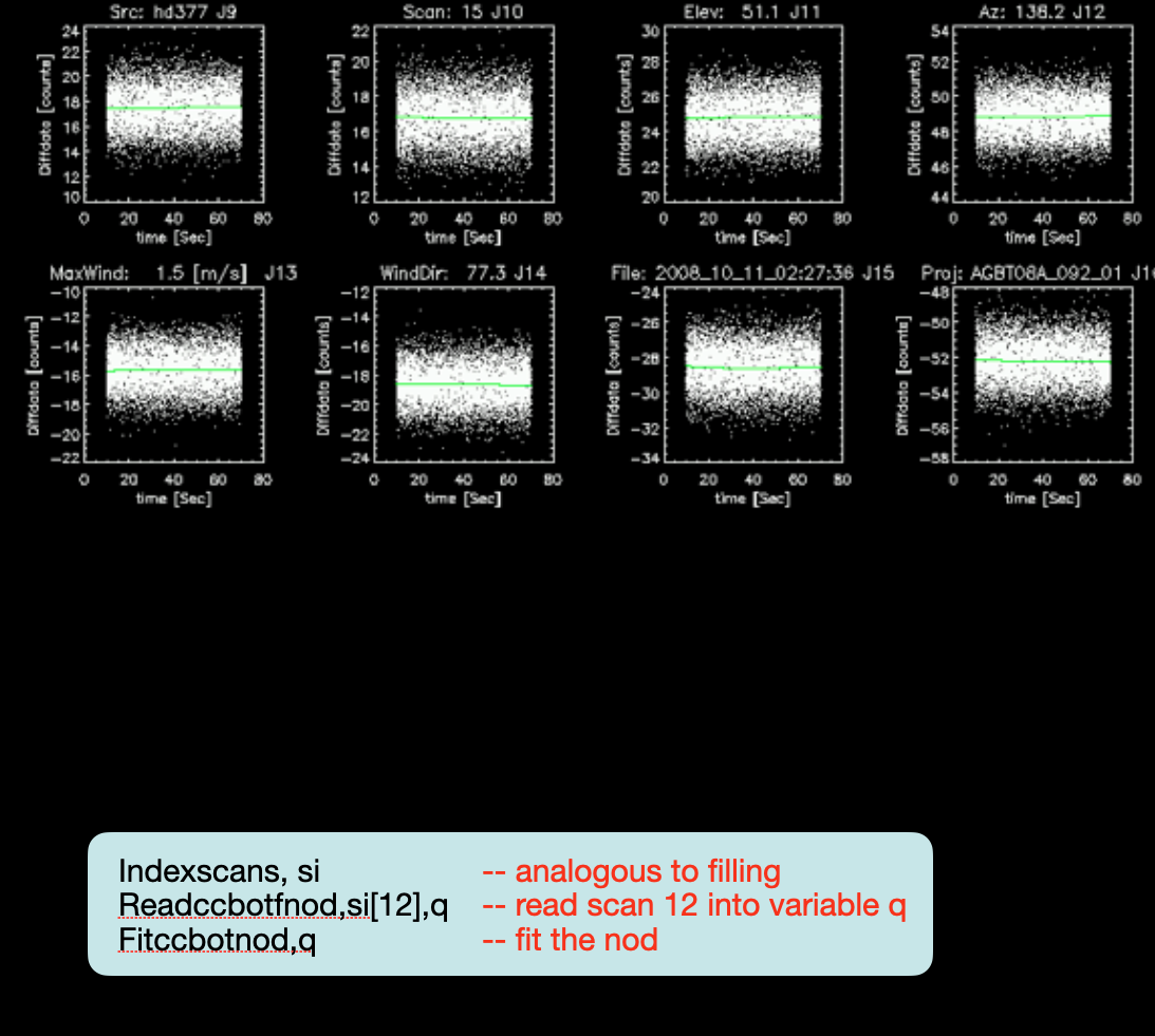
../../_images/ccbTutorial23feb09-013.png — Fig. 53 CCB OTF-NOD measurement of a weak (mJy-level) source under good conditions. The IDL commands used to obtain this plot are shown inset.#

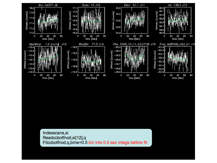
../../_images/ccbTutorial23feb09-014.png — Fig. 54 The same weak-source data, this time with the individual integrations binned into 0.5 second bins (using the optional argument `binwidth` in `fitccbotfnod`) so the thermal-noise scatter doesn’t dominate the automatically chosen y-axis scale. This better shows any gradients or low-level fluctutions in the beamswitched data (due, for instance, to imperfect photometric conditions). In this data they are not significant#

Here is an example data reduction session that provides a quick look at your data:

; ccb_reduction.pro
;
; set up global variables
;  don't write files or plots to disk...

proj='AGBT06A_049_09'
setccbpipeopts, gbtproj=proj, ccbwritefiles=0, gbtdatapath='/home/archive/science-data/tape-0016/'

; to use postprocessing scripts, set ccbwritefiles=1

; a good color table for the plots:
loadct, 12

; create an array indexing scan numbers
;  to file name
indexscans, si

; summarize the project
summarizeproject

; read a nod observation from scan 12
readccbotfnod, si[12], q

; fit the data, binning integrations to 0.5sec bins
fitccbotfnod, q, qfit, bin=0.5

; the resulting plot shows the differenced
;  data (white) and the fit to the data (green)
;  for each of 16 CCB ports. (the first 8 are blank)

; look at the next nod that just came in
;  this time calibrate to antenna temperature
;  before plotting
; First you need to derive a calibration, which
;  requires a scan with both cals firing independently.
; /dogain tells the code to solve for the calibration;
;  the results are stored in calibdat, which we can
;  pass into subsequent invocations of the calibration.
indexscans, si
readccbotfnod, si[13], q
calibtokelvin, q, /dogain, calibdat=calibdat
fitccbotfnod, q

; the scan index si must be updated to read in scans
;  collected after it was first created
indexscans, si
readccbotfnod, si[14], q

; and calibrate to kelvin using the information
;  we just derived
calibtokelvin, q, calibdat=calibdat

; fit/plot
fitccbotfnod,q

; et cetera...

Mapping data can also be imaged using the IDL tools:

; make a map from scans 7-10 using port 11 data 
;  (note the port must be specified; valid ports are
;   9-16)
img=makedcrccbmap([7,8,9,10],/isccb,port=11)

; replot the map
plotmap,img,/int

; make a png copy of it
grabpng,'mymap.png'

; save the map in standard FITS format--
saveimg,img,'mymap.fits'

This will be a beam-switched map. The beam-switching can be removed by an EKH deconvolution algorithm [Emerson et al., 1979] also implemented in the code. Your project friend will help you with this, if needed.

Performance#

Tests under excellent conditions show a sensitivity of 150µJy (RMS) for the most sensitive single channel (34 GHz), or 100µJy (RMS) for all channels combined together. These are the RMS of fully-calibrated, 70-second OTF-NODs on a very weak source. Typical reasonable-weather conditions are a factor of two worse.

Differences Between the CCB/Ka System and other GBT Systems#

There are a few differences between the CCB/Ka system and other GBT receiver/backend systems which users familiar with the GBT will want to bear in mind.

Because it is a direct detection system, the GBT IF system does not enter into observing.
The Ka/CCB gains are engineered to be stable (10% - 20% over months), so no variable attenuators are in the signal chain. Consequently there is no Balance() step.
To optimize the RF balance (for spectral baseline and continuum stability), the OMT’s have been removed from the Ka band receiver. It is therefore sensitive to one linear polarization per feed. The two feeds are sensitive to orthogonal linear polarizations (X and Y).
Feed orientation is \(45^\circ\) from the Elevation/cross-Elevation axes. All other receivers have feed separations that are parallel to the Elevation or cross-Elevation axes (except for the KFPA).
There are two cal diodes (one for each feed), and they are separately controlled (i.e., it is possible to turn one on and not the other). Cals are ON or OFF for an entire integration; they are not pulsed ON and OFF within a single integration.

CCB

Contents