VEGAS

VEGAS#

Overview#

The VErsatile GBT Astronomical Spectrometer (VEGAS) is an Field-Programmable Gate Array (FPGA) based spectrometer that can be used with any receiver except MUSTANG-2. It consists of eight independent spectrometers (banks) that can be used simultaneously. Eight-bit samplers and polyphase filter banks are used to digitize and generate the spectra – together they provide superior spectral dynamic range and RFI resistance. For details on the design of VEGAS, please consult http://www.gb.nrao.edu/vegas/report/URSI2011.pdf.

Todo

Move content of that pdf file here or link the file here or add a reference.

Observers can use between one and eight dual-polarization spectrometers (or banks) at the same time (see Fig.~ref{fig:vegasconfig}).

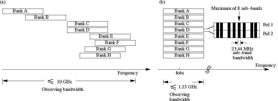
Each bank within VEGAS can be configured with a different spectral resolution, bandwidth, and number of spectral windows (subbands). However, the integration time (tint), switching period (swper), and the frequency switching offset (swfreq) values must each be the same for all banks. The resolution and bandwidth of all subbands in a single VEGAS bank must be identical, but the center frequencies may be set independently (within limits).

Although the individual banks could be arranged to cover 10 GHz of total bandwidth, the maximum bandwidth is typically limited to 4-6 GHz by filters in the GBT IF system (see your project friend for more information).

Todo

Either replace the reference to the project friend with the helpdesk or provide the information here.

All banks have the same switching signal (i.e., same switching period, same integration time, same frequency switching offset), which is controlled by spectrometer bank A. Each bank can be configured in one of the 29 modes listed in Table 15 below.

Table 15 VEGAS modes#
Mode	Bandwidth	Channels	Spectral resolution (kHz)	Minimum integration time^(b) (ms)	Max data rate^(a) at minimum integration time (MB\(^{-1}\))
Single sub-band modes
1^(c)	1500	1024	1465.00	1	32
2^(c)	1500	16384	92.00	2	187
3^(d)	1080	16384	66.00	4	130
4	187.5	32768	5.70	11	52
5	187.5	65536	2.90	22	52
6	187.5	131072	1.40	35	69
7	100	32768	3.10	12	51
8	100	65536	1.50	25	51
9	100	131072	0.80	40	69
10	23.44	32768	0.70	16	93
11	23.44	65536	0.40	33	93
12	23.44	131072	0.20	72	75
13	23.44	262144	0.10	134	93
14	23.44	524288	0.04	246	125
15	11.72	32768	0.40	27	93
16	11.72	65536	0.20	55	93
17	11.72	131072	0.10	123	62
18	11.72	262144	0.04	223	93
19	11.72	524288	0.02	447	93
8 sub-band modes^(e)
20^(c)	23.44	4096	5.70	6	12
21^(c)	23.44	8192	2.90	12	12
22^(c)	23.44	16384	1.40	35	8
23^(c)	23.44	32768	0.70	51	12
24^(c)	23.44	65536	0.40	97	13
25^(d)	16.9	4096	4.10	8	9
26^(d)	16.9	8192	2.10	17	9
27^(d)	16.9	16384	1.00	47	6
28^(d)	16.9	32768	0.51	69	9
29^(d)	16.9	65536	0.26	132	10

Footnotes for Table 15

(a): Maximum data rate is calculated for recording full polarization and all channels at the minimum integration period for one spectrometer. Each spectral value is represented by 4 bytes.
(b): The integration per switching state should be \(\ge\) the minimum integration. For example, if an observation uses 2 switching states, then the minimum integration will be 2 times the value listed in the table.
(c): For modes 20 \(\rightarrow\) 24 the subbands can be placed within the baseband bandwidth of 1500 MHz. The actual usable frequency range for modes 1 & 2 as well as modes 20 \(\rightarrow\) 24 is 1250 MHz.
(d): For modes 25 \(\rightarrow\) 29 the subbands can be placed within 1000 MHz. The actual usable frequency range for mode 3 as well as modes 25 \(\rightarrow\) 29 is 800 MHz.
(e): To use more than one subband, set vegas.subband=8, and the actual number of subband used is then defined by the number of frequencies provided.

In short:

Modes 1-19 provide a single subband per bank. Modes 1–3 have the following constraints on useable bandwidth:
- Modes 1-2: Have a useable bandwidth of 1250 MHz within the baseband bandwidth of 1500 MHz. The useable baseband frequency range is 150-1400 MHz.
- Mode 3: Has a useable bandwidth of 800 MHz within the baseband bandwidth of 1080 MHz. The useable baseband frequency range is 150-950 MHz.
Modes 20-29 provide up to eight subbands per bank. To use more than one subband, set subband=8, and the actual number of subbands used is then defined by the number of frequencies provided. All subbands must have equal bandwidths and be placed within the total bandwidth processed by that bank:
- Modes 20-24: Have a useable bandwidth of 1250 MHz within the baseband bandwidth of 1500 MHz. The useable baseband frequency range is 150-1400 MHz.
- Modes 25-29: Have a useable bandwidth of 800 MHz within the baseband bandwidth of 1080 MHz. The useable baseband frequency range is 150-950 MHz.

Each mode provides the polarization products XX, YY, and optionally XY,YX necessary for observations of polarized emission without requiring a reduction in the number of channels or sampling speed. VEGAS can also record only a single polarization for single-polarization receivers.

Data Rates#

The data rate for an individual bank can be calculated using

\[\text{Data Rate (GB/hr)} = 1.44 \times10^{-5} \cdot\dfrac{n_{channels}\times n_{spw}\times n_{stokes}\times n_{states}}{t_{int}\text{(seconds)}},\]

where \(n_{channels}\) is the number of channels per spectral window, \(n_{spw}\) is the number of spectral windows, \(n_{stokes}\) is the number of stokes parameters (2 for dual polarization, 4 for full polarization), \(n_{states}\) is the number of switching states (4 for frequency switching and 2 for total power), and \(t_{int}\) is the integration time. The total data rate for a project can be calculated by adding the data rates for each bank together.

IF Configuration#

The GBT IF system introduces some constraints on routing signals from the receivers to VEGAS.

Single beam receivers or a multi-beam receiver that has been configured to use a single beam may be routed to any or all of the VEGAS banks A \(\rightarrow\) H. No spectral resolution is gained with VEGAS by only using one beam of a multi-beam receiver.
Dual-beam configurations allow each beam to be routed to a maximum of 4 VEGAS banks.
When using 3–4 beams, each beam may be routed to up to a maximum of 2 VEGAS banks.
When using more than 5 beams, each beam may only be routed to a single VEGAS bank.
When using all 7 beams of the KFPA, each beam may be routed to a single VEGAS bank with an optional second copy of beam 1 being routed to the remaining VEGAS bank. This is known as the “7+1” mode of the KFPA.

Blanking#

While the observing system is switching between states (such as switching the noiseDiode on or off, switching frequencies, running doppler updates, etc…) the collected data is not valid, and thus must be ‘blanked’ by VEGAS. VEGAS allows the user to switch states frequently enough that the required blanking time can become a non-negligible percentage of the total observing time. For efficient observing, it is important to choose switching periods that are long enough for the total amount of blanking to be negligible. The amount of blanking per switching signal is dependent on the VEGAS mode used. Conservative values are shown in Table 16 and Table 17 for values with the noiseDiode turned either on or off. For a more thorough description of the appropriate switching periods for a given amount of blanking, and more accurate estimates of the minimum switching periods we refer the interested reader to Kepley et al. [2014].

Table 16 Minimum recommended switching periodes (`swper`) with VEGAS for observations that **use a noise diode**.#
Mode	Total power (tp)	Frequency switching^(a) (sp)
	Nominal^(b) swper (s)	Nominal^(c) swper (s)	\(\nu_{min}\) ^(d) (GHz) swper=1.52s	Mapping^(e) swper (s)
1	0.01	0.4	115.0	0.4
2	0.028	0.4	115.0	0.4
3	0.04	0.4	115.0	0.4
4	0.028	0.4	115.0	0.4
5	0.0559	0.4	115.0	0.4
6	0.1118	0.4318	115.0	1.52
7	0.0524	0.4	115.0	0.4
8	0.1049	0.4249	115.0	1.52
9	0.2097	0.5297	59.6	1.52
10	0.2237	0.5437	54.4	1.52
11	0.4474	0.8948	16.5	1.52
12	0.8948	1.7896		1.7896
13	1.7896	3.5791		3.5791
14	3.5791	7.1583		7.1583
15	0.4474	0.8948	16.5	1.52
16	0.8948	1.7896		1.7896
17	1.7896	3.5791		3.5791
18	3.5791	7.1583		7.1583
19	7.5383	14.3166		14.3166
20	0.028	0.4	115.0	0.4
21	0.0559	0.4	115.0	0.4
22	0.1118	0.4318	115.0	1.52
23	0.2237	0.5437	54.4	1.52
24	0.4474	0.8948	16.5	1.52
25	0.0388	0.4	115.0	0.4
26	0.0777	0.4	115.0	1.52
27	0.1553	0.4753	89.7	1.52
28	0.3107	0.6307	33.8	1.52
29	0.6214	1.2428	8.6	1.52

Footnotes for Table 16

(a): When frequency switching, switching periods must always be \(\ge\) 0.4 seconds due to the settling time of the LO1
(b): Recommended minimum switching period (swper) for total power observations with a noise diode (swtype='tp'). These values will yield less than 10% blanking overall.
(c): Recommended minimum switching period for frequency-switched observations with a noise diode (swtype='sp'). These values will yield less than 10% blanking in the first state of the switching cycle as well as less than 10% blanking overall.
(d): The minimum recommended switching period is 1.52 seconds when Doppler tracking frequencies above \(\nu_{min}\).
(e): Recommended minimum switching period (swper) for Doppler-tracked, frequency-switched observations with a noise diode (swtype='sp'). These values will yield less than 10% blanking in the first state of the switching cycle as well as less than 10% blanking overall. This switching period will result in less than 10% of the data being blanked. These values assume that the maps are sampled at twice Nyquist in the scanning direction and that there are four integrations per switching period when Doppler tracking.

Table 17 Minimum recommended switching periodes (`swper`) with VEGAS for observations that **do not use a noise diode**.#
Mode	Total power (tp)		Frequency switching^(a) (sp)
	Nominal ^(b) swper (s)	Mapping ^(c) swper (s)	Nominal^(d) swper (s)	\(\nu_{min}\) ^(e) (GHz) swper=0.76s	Mapping ^(f) swper (s)
1	0.0005	0.001	0.4	115.0	0.4
2	0.0014	0.0028	0.4	115.0	0.4
3	0.002	0.004	0.4	115.0	0.4
4	0.01	0.0114	0.4	115.0	0.4
5	0.0199	0.0227	0.4	115.0	0.4
6	0.0301	0.0357	0.4	115.0	0.76
7	0.0102	0.0128	0.4	115.0	0.4
8	0.0203	0.0256	0.4	115.0	0.76
9	0.0301	0.0406	0.4	115.0	0.76
10	0.0056	0.0168	0.4	115.0	0.76
11	0.0112	0.0336	0.4474	33.1	0.76
12	0.028	0.0727	0.8948		0.8948
13	0.0447	0.1342	1.7896		1.7896
14	0.0671	0.2461	3.5791		3.5791
15	0.0056	0.028	0.4474	33.1	0.76
16	0.0112	0.0559	0.8948		0.8948
17	0.0336	0.123	1.7896		1.7896
18	0.0447	0.2237	3.5791		3.5791
19	0.0895 or ^(g) 0.38	0.4474	7.1583		7.1583
20	0.0051	0.0065	0.4	115.0	0.4
21	0.0101	0.0129	0.4	115.0	0.4
22	0.0301	0.0357	0.4	115.0	0.76
23	0.0405	0.0517	0.4	115.0	0.76
24	0.0755	0.0979	0.4474	33.1	0.76
25	0.007	0.009	0.4	115.0	0.4
26	0.0141	0.018	0.4	115.0	0.76
27	0.0398	0.0476	0.4	115.0	0.76
28	0.0544	0.0699	0.4	68.6	0.76
29	0.101	0.132	0.6214	17.1	0.76

Footnotes for Table 17

(a): When frequency switching, switching periods must always be \(\ge\) 0.4 seconds due to the settling time of the LO1
(b): Recommended minimum switching period (swper) for total power observations that do not use a noise diode (swtype='tp_nocal'). This value is equivalent to the hardware exposure value for VEGAS.
(c): Recommended minimum switching period (swper) for total power OTF mapping observations that do not use a noise diode (swtype='tp_nocal') when Doppler Tracking. These values will yield less than 10% blanking overall and assume that the maps are sampled at twice Nyquist in the scanning direction and that there are four integrations per switching period.
(d): Recommended minimum switching period for frequency-switched observations that do not make use of a noise diode (swtype='sp_nocal'). These values will yield less than 10% blanking in the first state of the switching cycle as well as less than 10% blanking overall.
(e): The minimum recommended switching period is 0.76 seconds when Doppler tracking frequencies above \(\nu_{min}\).
(f): Recommended minimum switching period (swper) for Doppler-tracked, frequency-switched OTF mapping observations without a noise diode (swtype='sp_nocal'). These values will yield less than 10% blanking in the first state of the switching cycle as well as less than 10% blanking overall. This switching period will result in less than 10% of the data being blanked. These values assume that the maps are sampled at twice Nyquist in the scanning direction and that there are four integrations per switching period.
(g): For mode 19 this value is 0.0895/0.38 seconds for observations below/above 10.3 GHz when Doppler tracking.

Monitoring VEGAS observations#

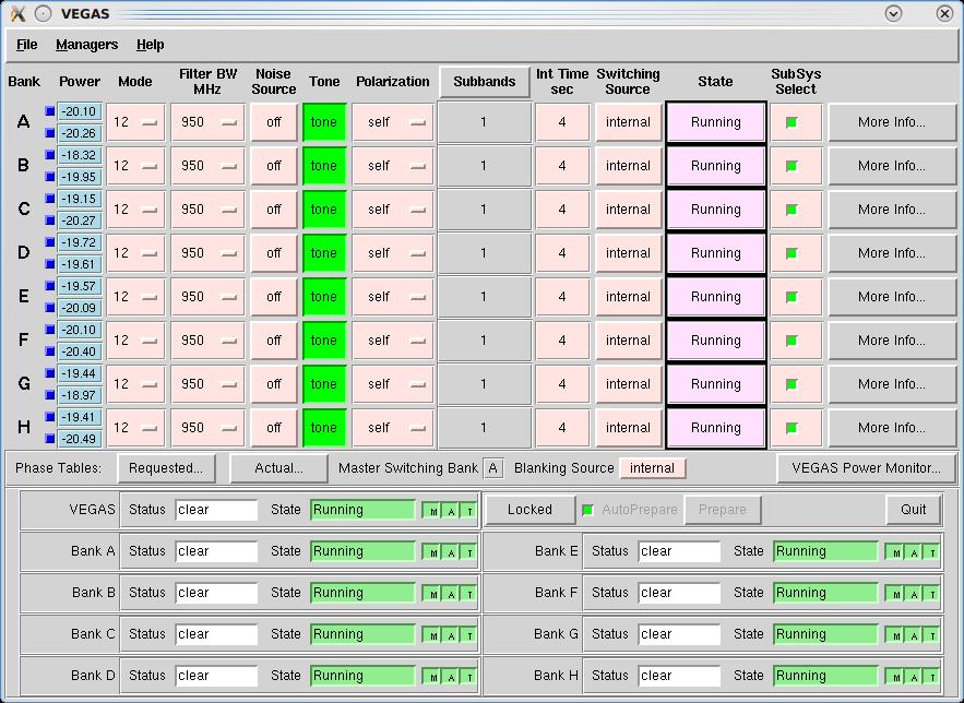
The Spectral Line tab in the Astrid Data Display is not fully capable of displaying VEGAS observations in real time (it will display passbands at the end of a scan, and may be used in offline mode). Rather, there are two monitoring tools that you may find useful as a VEGAS user:

The CLEO VEGAS screen#

See the CLEO VEGAS description for more information.

VEGAS Data Monitor (VEGASDM)#

The VEGAS Data Monitor (VEGASDM) provides a real-time display of the current total power level as measured by the VEGAS ADC, as well as a histogram of the distribution of ADC counts. VEGASDM may be launched by:

source /home/gbt/gbt.bash  # (or .csh)
VEGASDM

or by clicking the VEGAS Power Monitor... button from the CLEO VEGAS screen.

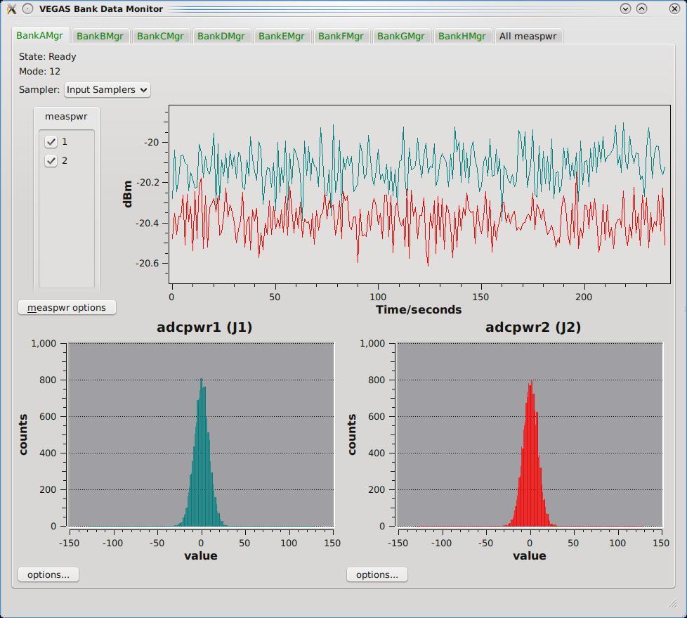
VEGASDM has nine tabs, one for each Bank, and one overview tab. If a Bank is active, the tab label will be green, otherwise it will be red. Each Bank tab shows whether the Bank is in the running state, and what mode it is in. The upper plot shows the total power from each polarization as a function of time, while the lower two plots show the distribution of ADC counts for each polarization. If VEGAS is balanced correctly, the ADC counts should be approximately Gaussian, centered around zero, with a full-width half maximum of approximately 25-50 counts. If the ADC counts are very centrally peaked, there is not enough power going into VEGAS, while if the ADC counts have peaks at +/- 127 counts, VEGAS is being over-driven.

The final tab of VEGASDM gives an overview plot of the total power for all eight banks on a single screen.

The Online Filler and filling VEGAS data using SDFITS#

VEGAS writes Engineering FITS files. Once a scan is over, the Filler reads these files, combines the data with metadata from the Antenna and other FITS files, and produces a single-dish (SDFITS) file. This can be done automatically, by the on-line filler, or manually by the Observer. Due to the significantly higher data rate, and some other features of VEGAS, the filling process requires some oversight by the user.

The Online Filler#

The online filler will make every attempt to fill the SDFITS file automatically. In this case, a file will be produced in /home/sdfits/<project> and GBTIDL can connect to it automatically using the online, or offline commands. There are some caveats, however.

Because of the way VEGAS writes its data, the filler cannot start filling until the scan has finished.
For large scans, the filler could potentially fall behind the data acquisition process. To avoid this, the filler will skip scans that it cannot keep up with. The rule is:
```
If (integrationTime / totalNumberOfSpectraPerIntegration) < 0.00278s
    skip the scan
Except if (integrationLength >= 0.9s) it will be filled
```

The total number of spectra per integration is the total across all banks. So, for example, 2 banks, 8 subbands, 2 polarizions and 4 switching states (e.g. frequency switching with calibration) will produce 2*8*2*4 = 128 spectra, and so if the integration time is <0.356s the online filler will not fill that data. The 0.9s limit is because for that integration time the online filler can almost keep up even in the worst case, and interscan latencies, pauses for pointing and focus scans, and so on will nromally allow it time to catch up. The online filler prints a summary in /home/sdfits/<project>/<project>.log indicating what scans were filled, had problems and were skipped, and if any data was skipped because the data rate was too fast.

The decision on whether to fill or not is made independently for each bank. For cases where the integration time is close to the limit it’s possible that some banks might be filled while others are not filled for the same scan if the number of subbands or the number of polarizations vary across the banks. The summary log file will indicate when this happens.

If observers are concerned about the interpolation across the center channel (see S~ref{sec:vegas_spike}) they can turn that off in sdfits by using the -nointerp option.

Filling Offline#

You may wish to (re-)fill your data offline. In this case, you may use the SDFITS filler program in the standard manner. Note however, that the actual VEGAS data is stored to a high-speed (lustre) file system. For a current list of lustre client machines please see https://greenbankobservatory.org/portal/gbt/processing/#data-reduction-machines

If you try to fill data without being logged into a lustre client, the filler will fail with the error message:

VEGAS data expected but not found, this workstation is not a lustre client.
For a list of public lustre client workstations see:
http://www.gb.nrao.edu/pubcomputing/public.shtml

In this case, ssh to a lustre client (using the domain .gb.nrao.edu), and fill your data there.

Filling using sdfits directly (instead of the output online sdfits) might also be useful if there are a lot of spectra to be processed in GBTIDL simply because it improves the response times in GBTIDL if there are not as many spectra to search through. So if there’s a convenient way to divide up the scans, then this sort of syntax works (see sdfits -help for more details):

sdfits -backends=vegas -scans=<scan-list> <PROJECT_SESSION> <OUTPUT_PREFIX>

<scan-list> is a list of comma separated scans to fill using colons to denote ranges e.g., -scans=1,4:6,10 would fill scans 1,4,5,6 and all scans from 10 onwards
<PROJECT_SESSION is what you’d expect, e.g. AGBT14A_252_04
<OUTPUT_PREFIX> is the leading part of the output directory name, e.g. scan5to25 would result in a directory named scan5to25.raw.vegas

Instrumental Features and their Cure#

The architecture of the VEGAS hardware, specifically the architecture of the Analog to Digital Converter (ADC), results in some characteristic features in the VEGAS spectrum. Specifically, these are:

a strong spurious single-channel wide spike at the exact center of the ADC passband – the so-called center spike.
weak single-channel wide spurs at various locations in the bandpass – the 32 spurs.

The Spike#

The center spike is caused by the FPGA clock. By default, the center spike is interpolated over by the SDFITS filler by taking the mean of the adjacent channel on either side of the spike. The center spike is also interpolated-over by the real-time spectrum display. We have chosen to interpolate over this spike as it is omnipresent, and can cause problems for data reduction (such as system temperature calculations). If you are concerned about this process, you may shift your line from the center of the passband using the deltafreq keyword in your astrid script.

The Spurs#

When attempting to search for RFI with VEGAS by running a high-pass filter through the data, significantly more spikes/spurs were found than naively expected. These spurs could be found in the same bins in relatively RFI free wavelengths, such as Q band. The spurs appear at the same location (in bin space) for a given mode and have relatively stable amplitudes. These faint spurs are not always directly visible in the data, but became clear when high-pass filtered, as shown here:

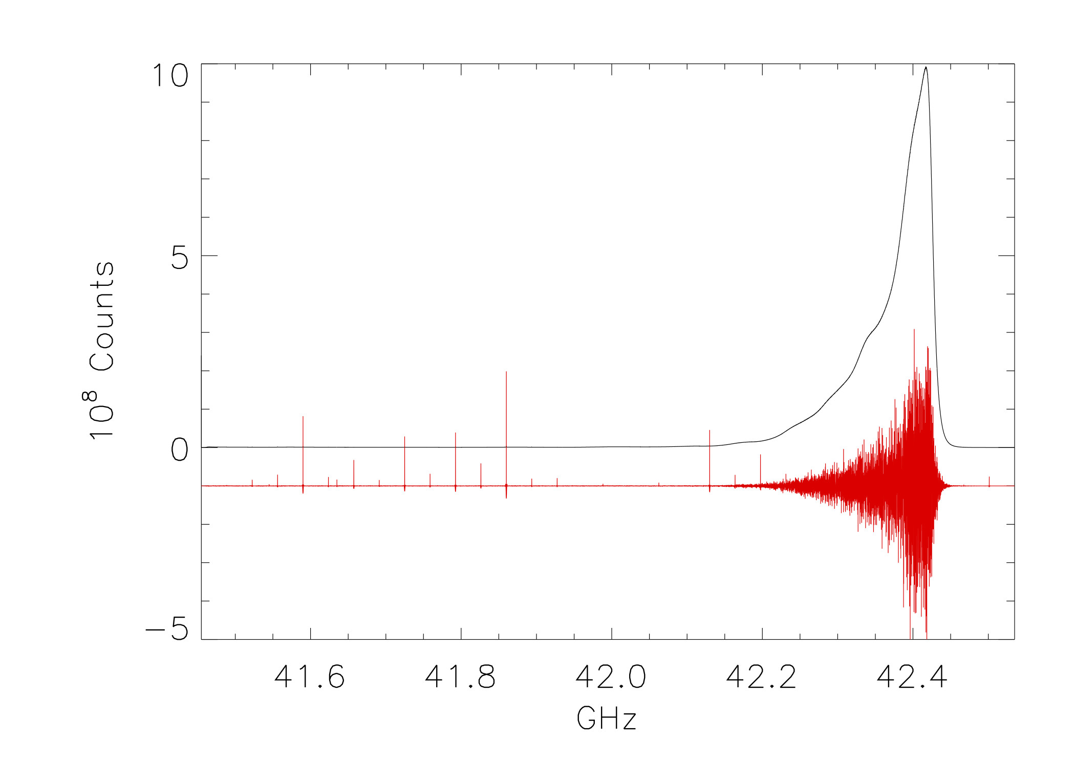
../../_images/vegas_raw_with_digital_filt.jpg

After significant testing, it was determined that these spurs are below the spurious-free dynamic range of -60dBc specified by the manufacturer, and cannot be fully removed. In overly simplistic terms, the spurs are caused by the leaking of the FPGA clock into the four interleaved ADCs.

These spurs are relatively stable and will remain constant (for a given mode) and the magnitude of the spurs is relatively constant. These features are also quite small by most standards (Spurious Free Dynamic Range no more than -60dBc), but nevertheless can be problematic when looking for faint narrow features. The stability of these features allows them to be removed by standard data practices (such as position and/or frequency switching), but they are an added noise source which can bleed through to the final product. Due to the limited and often negligible effect of these spurs, we do not automatically interpolate across them, but let the user decide how to handle those channels.

Known Bugs and Features#

Data is not filling#

The online filler checks for project changes when it is not actively filling a scan. This means that if the previous project was a VEGAS one and it ended on a long scan, the filler may still be filling that project when the VEGAS scan has finished in your project. If you suspect that this is the case, the only solution is to ask the Operator to restart the online filler task.

All data can still be accessed in GBTIDL by running SDFITS offline.

There is a square wave and/or divot in my VEGASDM display#

The samples which are taken to produce the VEGASDM total power display run asynchronously to the switching signals. Hence, the sampling may occur during the Cal on phase at one point in time, and then drift into the Cal off phase sometime later. This may produce an apparent square wave in the VEGASDM output, with an amplitude of a few tenths of a dB, and a period of seconds.

Similarly, it is possible for the VEGASDM data to be acquired when the LO is updating (e.g. during a Doppler track). These data are blanked in the true VEGAS spectral data acquisition, but may cause drop-outs in the VEGASDM samples.