
Cyclic Spectroscopy#
Overview#
The GBT offers a CS backend system which produces periodic spectra (related to the cyclic spectrum via a Fourier transform) in close-to-real time (the operation of the system is described in more detail below). It operates simultaneously with VEGAS to produce both traditional coherent-dedispersion fold-mode pulsar data along with periodic spectra. CS can be used with any GBT receiver other than MUSTANG2.
The CS backend shares some components with VEGAS. Specifically, the
VEGAS ROACH2 boards are used to perform a first-stage channelization
via a polyphase filterbank (PFB). Note that the number of PFB
channels (denoted by \(n_{\rm pfb}\)) is the same as the number of
frequency channels in traditional VEGAS pulsar data. These coarsely
channelized baseband data are sent via ethernet to both VEGAS (where
they are processed in real-time to produce traditional data products)
and to a dedicated CS processing cluster. CS can be used with the
100, 200, 800, and 1500 MHz-bandwidth coherent dedispersion modes of
VEGAS, producing one, two, eight, or eight data streams. Each stream
is a duplicate copy of the data sent to and processed on a VEGAS Bank.
CS streams retain this nomenclature (i.e. the data stream associated
with VEGAS Bank A is also labeled A). Fig. 40
provides a schematic overview of the CS system and its shared
components with VEGAS.
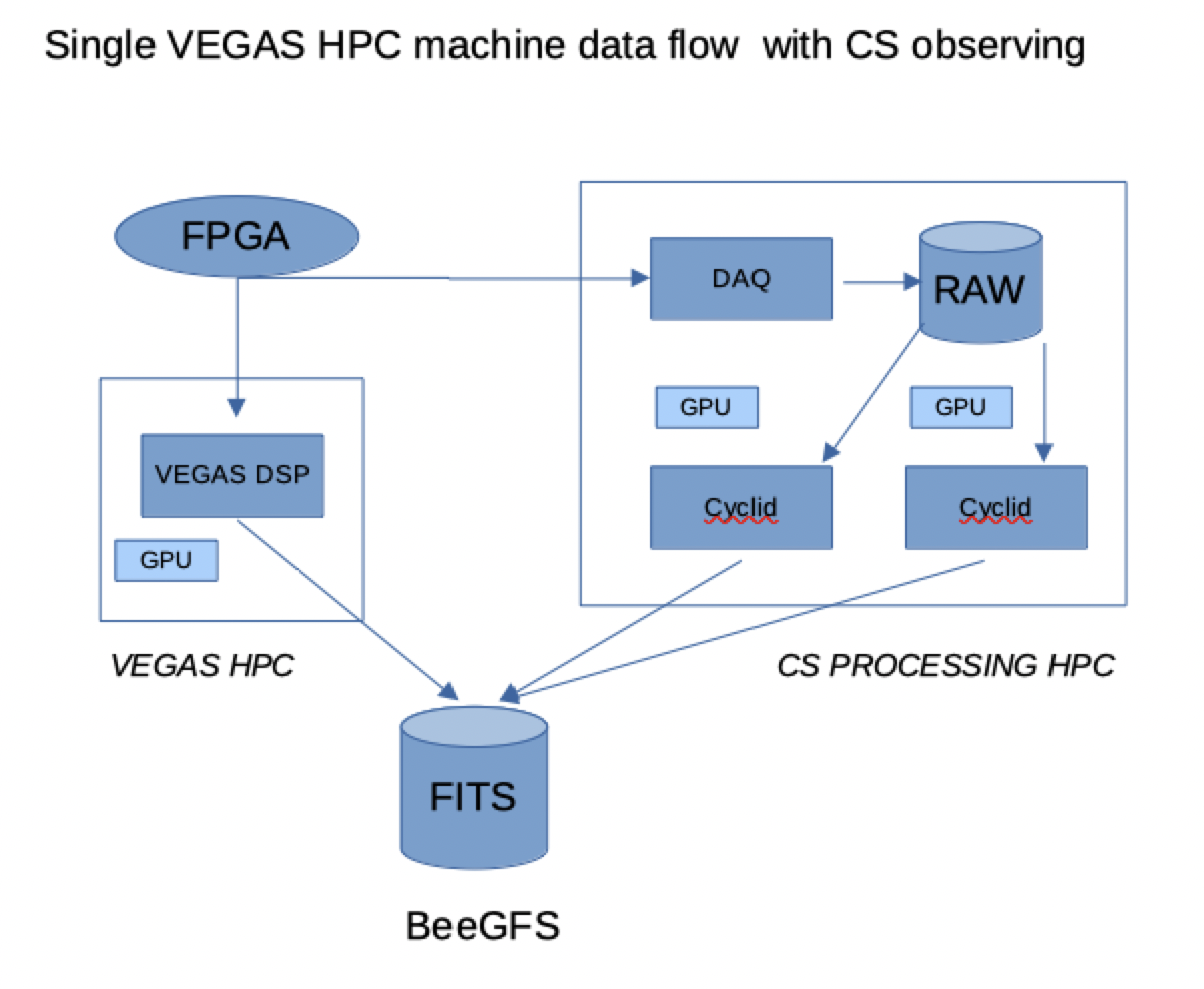
Fig. 40 A simplified, schematic overview of the CS system and its relationship to VEGAS. Note that only a single CS stream/VEGAS Bank is depicted here. Data from a VEGAS ROACH2 FPGA is multi-cast over Ethernet to both a VEGAS HPC (where the digital signal is processed using traditional techniques) and to a CS processing HPC. Raw baseband data from a CS data stream is stored on dedicated disks and processed using custom GPU-accelerated software (known as cyclid). Two scans from each VEGAS Bank/CS data stream can be processed simultaneously. Both VEGAS and the CS system write final FITS data products to the BeeGFS mass file store.#
The baseband data are temporarily saved to disk on the CS cluster, and processed after a scan ends. Each data stream has its own, dedicated storage disk and two dedicated GPUs that are used to process data. This involves using CS to further channelize the data to achieve finer frequency resolution, while still maintaining pulse phase resolution. The additional channelization factor is denoted by \(n_{\rm cyc}\) and the number of pulse phase bins is denoted by \(n_{\rm bin}\). The final frequency resolution is given by
where BW is the total bandwidth.
Processing begins automatically once a scan ends. After periodic spectra have been produced they undergo automated quality checks and, after passing, the baseband data are automatically deleted, freeing space for subsequent observations. The time it takes to produce period spectra depends on the combination of observing parameters but is limited to \(\leq 2\times\) the length of the observation. Data acquisition and post-processing status are monitored via a browser-based interface.
Allowable Observing Parameters#
The storage disks associated with each data stream have a maximum capacity of 16 TB each. This is sufficient to record up to approximately 6 hours of data when using 1500 MHz or UWBR modes, and 11 hours of data when using 100, 200, or 800 MHz bandwidth modes. There are also two GPUs used to process data from each stream after a scan ends. To ensure that the CS system can be used continuously without exceeding the capacity of the local storage or negatively impacting system performance, there are restrictions on the maximum length of an individual scan and the time it takes to process a scan:
An individual scan is limited to \(\leq\) one hour.
The time to process a scan is limited to \(\leq\) twice the scan length.
The latter restriction limits the allowable combination of PFB channel bandwidth, the final frequency resolution of the periodic spectrum, and the pulse phase resolution. Allowable parameter combinations are shown in Table 21.
\(n_{\rm pfb} \downarrow\) |
\(n_{\rm bin} \rightarrow\) |
32 |
64 |
128 |
256 |
512 |
1024 |
2048 |
|---|---|---|---|---|---|---|---|---|
100 MHz Bandwidth Modes |
||||||||
64 |
512 |
512 |
512 |
256 |
256 |
128 |
64 |
|
128 |
512 |
512 |
256 |
256 |
128 |
64 |
64 |
|
256 |
512 |
256 |
256 |
128 |
64 |
64 |
32 |
|
512 |
256 |
128 |
128 |
64 |
64 |
32 |
||
200 MHz Bandwidth Modes |
||||||||
64 |
256 |
256 |
256 |
256 |
256 |
128 |
128 |
|
128 |
512 |
512 |
512 |
256 |
256 |
128 |
64 |
|
256 |
512 |
512 |
256 |
256 |
128 |
64 |
64 |
|
512 |
512 |
256 |
256 |
128 |
64 |
64 |
32 |
|
1024 |
256 |
128 |
128 |
64 |
64 |
32 |
||
800 MHz Bandwidth Modes |
||||||||
32 |
32 |
32 |
64 |
64 |
32 |
32 |
32 |
|
64 |
128 |
128 |
128 |
128 |
128 |
128 |
128 |
|
128 |
128 |
256 |
128 |
128 |
128 |
128 |
128 |
|
256 |
256 |
256 |
256 |
256 |
256 |
128 |
128 |
|
512 |
512 |
512 |
512 |
256 |
256 |
128 |
64 |
|
1024 |
512 |
512 |
256 |
256 |
128 |
64 |
64 |
|
2048 |
512 |
256 |
256 |
128 |
64 |
64 |
32 |
|
4096 |
256 |
128 |
128 |
64 |
64 |
32 |
||
1500 MHz Bandwidth Modes |
||||||||
64 |
64 |
16 |
32 |
64 |
16 |
16 |
16 |
|
128 |
64 |
64 |
64 |
64 |
64 |
64 |
64 |
|
256 |
128 |
128 |
128 |
128 |
128 |
128 |
64 |
|
512 |
256 |
256 |
128 |
128 |
128 |
64 |
64 |
|
1024 |
256 |
256 |
256 |
128 |
128 |
64 |
16 |
|
2048 |
256 |
256 |
128 |
128 |
64 |
32 |
8 |
|
4096 |
256 |
128 |
64 |
64 |
16 |
4 |
||
4500 MHz Bandwidth UWBR Modes |
||||||||
768 |
128 |
128 |
128 |
128 |
128 |
128 |
64 |
|
1536 |
256 |
256 |
128 |
128 |
128 |
64 |
64 |
|
3072 |
256 |
256 |
256 |
128 |
128 |
64 |
16 |
|
6144 |
256 |
256 |
128 |
128 |
64 |
32 |
8 |
|
12288 |
256 |
128 |
64 |
64 |
16 |
4 |
||
Using Cyclops to Monitor Your CS Observations#
During CS observations you should make use of the VPM observing tools relevant for coherent dedispersion fold and calibration modes. The CS backend has its own tools for monitoring observations, but they differ from the typical GBT backend because of the unique architecture of the CS backend, which shares much of its data acquisition infrastructure with VEGAS and processes data offline (rather than in real time). Most notably, the CS backend does not have a CLEO application that interfaces with a software Manager. In addition, while errors during the data acquisition stage will trigger messages that are displayed in the CLEO Message application, errors during the offline processing stage will not appear in CLEO Message.
Instead, CS observations are monitored using Cyclops, a browser-based interface that “keeps an eye on things”. Cyclops can only be accessed from a computer on the GBO internal network, and also requires a login using your my.nrao.edu credentials. Cyclops allows users to monitor ongoing data acquisition and the status of offline processing. Note that you will only be able to view information for GBT projects on which you are a PI or Co-I. We detail various features of Cyclops in the sections below.
The Cyclops Dashboard#
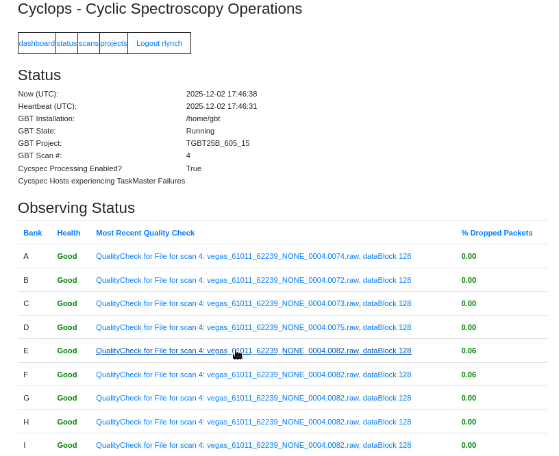
Fig. 41 The Cyclops Dashboard. Observers should use this page to check on the overall health of the system. Note that click on a quality check link takes one to a detailed overview of the quality of the last scan.#
A screen shot of the dashboard page is shown in Fig. 41. This page gives a high level overview of the health of the CS backend. Observers should note the following information.
The “Now” and “Heartbeat” timestamps should be relatively current (within one minute of the last page refresh). If they are not, the text will turn red.
The “GBT State”, “GBT Project”, and “GBT Scan #” should reflect the current state of the GBT.
“Cycspec Obs Now?” should be True when you are taking CS data.
“Cycspec Processing Enabled” should always be True during normal operations.
All active Banks should have a Health status of Good and Dropped Packets percentage very close to zero (\(< 0.1%\)).
Notify the GBT operator if you notice any problems. Clicking on a Quality Check link will bring you to a page showing more detailed information about the quality of the data (see below for details).
The Cyclops Status Page#
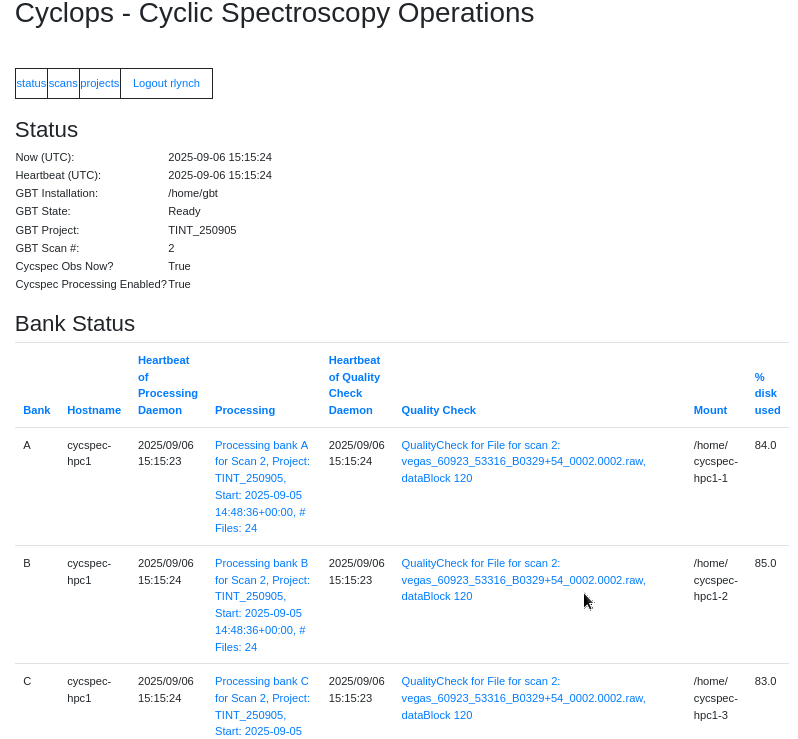
Fig. 42 The Cyclops Status page. This provides a snapshot of the overall status of the system. Note that additional information is shown lower in the page.#
A screen shot of the status page is shown in Fig. 42. The first section is the same as on the Dashboard. The next section shows more detailed information about the status of the data stream associated with each VEGAS Bank. Note that clicking on a column heading will sort that column, and clicking it again will sort it in the opposite sense (this is true throughout Cyclops). Observers should note the following information.
Only data streams associated with active VEGAS Banks should have current information. Depending on the observing bandwidth, not all Banks may be active.
The Processing Daemon and Quality Check Daemon Heartbeats should be current. They will turn red if they are not.
Observers can click on the links under Processing and Quality Check to see more information about the most recently processed and recorded data for that Bank, but remember that this may not be for your current scan if that Bank is not active.
Under normal operations the storage disks should always have adequate space, but if you notice that they are approaching 100% you should inform the GBT operator.
After the Bank Status section there is a table showing information about recent VEGAS scans. The columns contain information on various aspects of the scan and configuration. Observers can also see the current Processing State of the scan and whether the baseband data have been deleted. Clicking on the scan number will take you to a page showing more detailed information on that scan, and clicking on a project ID will take you to a page summarizing the project and session.
The Cyclops Projects Page#
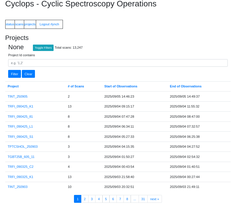
Fig. 43 The Cyclops Projects page. Clicking on a link will take you to a page with project-specific details.#
A screen shot of the status page is shown in Fig. 43. Observers can filter based on specific strings in the project ID. Clicking on a project ID will take you to a project-specific page with more details (shown in Fig. 44). From this page, observers can filter for specific scans and view detailed information on each scan. The information presented for each scan is the same as in the Scans table in the main Status page. Again, clicking on a scan number will take you to a page with detailed information on that scan.
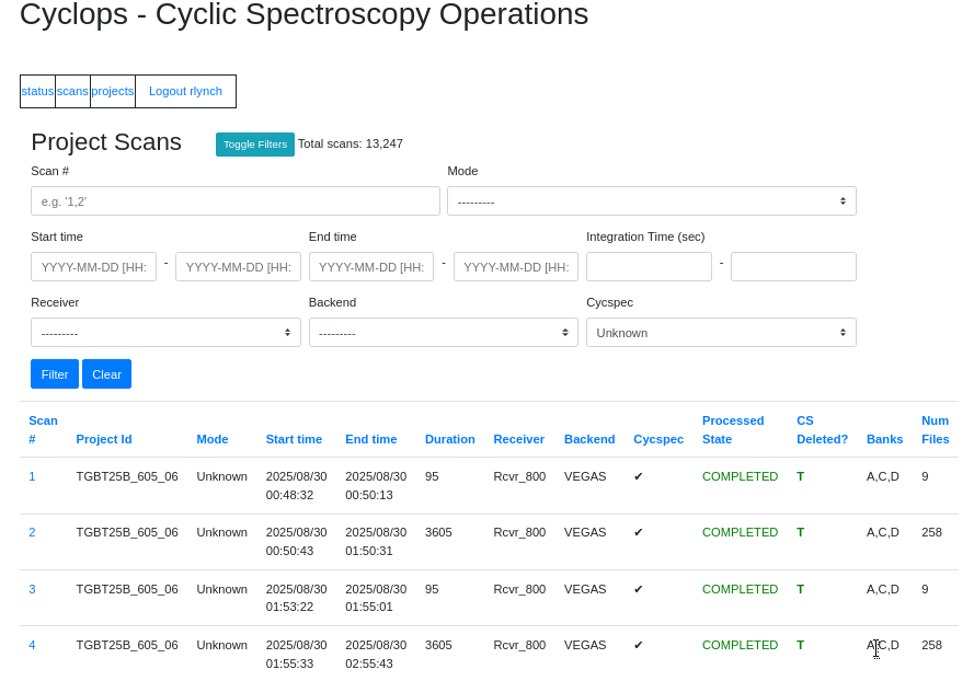
Fig. 44 A Cyclops page with detailed information about a single project. Clicking on a link will take you to a page with project-specific details. Clicking on a scan will take you to a page with more detailed information about that specific scan.#
The Cyclops Scans Pages#
Screenshots of the scan pages are shown in Fig. 45 (all scans) and Fig. 46 (scans associated with a specific project).
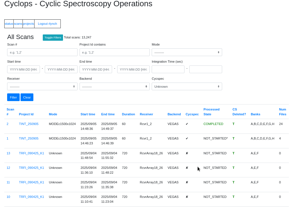
Fig. 45 The Cyclops Scans page. This contains information about all CS scans for all projects.#
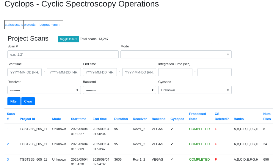
Fig. 46 Cyclops scans associated with a specific project.#
Clicking on a scan number will take you to a scan-specific page with more details (shown in Figs. Fig. 47 and Fig. 48). The first section shows the full path, file number, bank number, file type, creation time, size (in bytes), and data-taking status for each baseband file associated with this scan, as well as whether or not the baseband file has been deleted. The next section contains quality check information about the baseband data (see Fig. 49).
The most useful feature is the ability to click on a quality check ID, which will take you to a page showing various metadata about the scan and some visualizations of the baseband data themselves. Observers should not the following:
The OBSBW, OBSFREQ, and OBSNCHAN values should agree with what is shown in the vpmStatus tool for this bank and scan.
DROPT is a counter for dropped packets (i.e., data that has been lost because some aspect of the CS system can’t keep up with the incoming data stream). It has the same meaning as on the Dashboard and should be very close to zero.
The two plots show histograms of the 8-bit signed integer baseband values for each polarization, and the RMS in each frequency channel (which is proportional to the total power bandpass). The histograms should be approximately Gaussian in shape with an RMS of about 20 counts. Similarly, the bandpass RMS should also be about 20 counts in each channel. Note, however, that the total power varies significantly over the operating frequency range of several receivers, so variations on the order of \(\pm 15\) counts are not abnormal. Also, frequency ranges with relatively little power (e.g. near the receiver band edges, or where there is an RFI filter) will have little power and therefore a smaller RMS. Conversely, frequency ranges with strong RFI may have higher power and therefore a larger RMS. In general, if you are using a well-tested value of vegas.scale (see here) then the levels shown in these plots should be close to optimal. If you have doubts, contact the GBT operator.
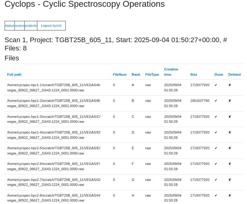
Fig. 47 A Cyclops page showing detailed information about a specific scan (continued in the next figure).#
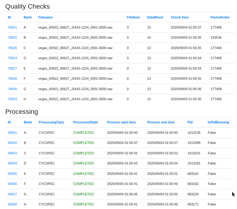
Fig. 48 Continuation of the detailed scan page in Cyclops.#
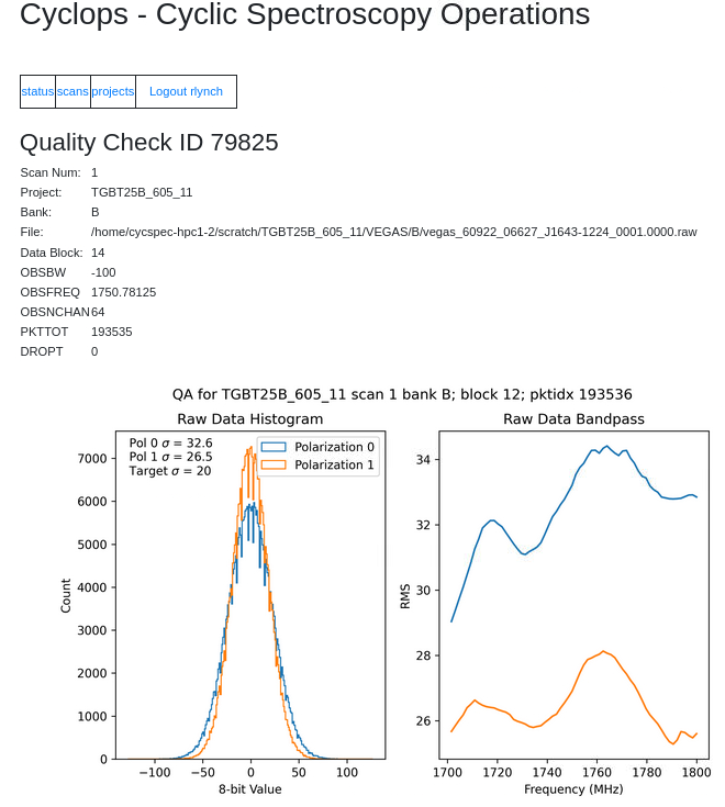
Fig. 49 A Cyclops quality check page. Observers should make sure that the baseband sample histogram and bandpass plots have appropriate RMS and power. See the text for details.#
The next section shows the processing status for each bank associated with this scan. Clicking on the processing ID will take you to a page showing the output of the processing software. Observers generally do not need to pay attention to this.
Accessing Your Data#
CS data will begin to appear shortly after a scan ends, and processing should finish within \(2\times\) the scan duration (e.g. a 1-hour long scan will finish processing within 2 hours).
Data are written in the PSRFITS format to the BeeGFS file system and can be accessed from any of the machines listed as `BeeGFS clients <https://www.gb.nrao.edu/pubcomputing/public.shtml`_ (e.g. euclid or thales). The directory and file naming conventions are very similar to those used by VEGAS. Files are written to project-specific directories of the form noindent /stor/gbtdata/<projectID>/CYCSPEC/<bankID> where <projectID> is your GBT project code with the session number in Astrid appended, e.g. AGBT18A_100_01, and <bankID> is the one-letter bank name.
File names follow the format vegas_<MJD>_<secUTC>_<sourceName>_<scanNumber>_<fileNumber>.fits where <MJD> is the modified Julian date of the observation, <secUTC> is the number of seconds after midnight UTC at the start of the scan, <sourceName> is the source name as identified from the Antenna manager, <scanNumber> is the scan number within the current Astrid session, and <fileNumber> is the file number within the current scan (long scans are broken across multiple files to avoid any one file from being very large). <secUTC> is a zero-padded five-digit integer and <scanNumber> and <fileNumber are zero-padded four-digit integers.
Note that the data written to /stor/gbtdata are the unmerged data from each bank. A cron job runs each hour which combines these data into files that cover the full observing bandwidth. These files are written to /stor/pulsar/gbtdata under project-specific directories. These merged data are what most observers will ultimately want to use for their science.
CS data are archived and are subject to standard GBO data management policies.
Additional Considerations#
Observers should be aware of the following.
VEGAS uses a critically sampled PFB and each channel is tapered to minimize interchannel spillover. As such, there are gaps between PFB channels in the periodic spectrum. The half-power width of these gaps is approximately 9% of the PFB channel bandwidth.
The cyclic spectrum is only valid when \(|f| < \mathrm{BW_{\rm pfb}}/2 - | \alpha/2|\) where \(\mathrm{BW_{\rm pfb}}\) is the PFB channel bandwidth, \(\alpha = k/P\), \(P\) is the pulsar period, and \(k = 0 \dots n_{\rm bin}\). This imposes a limit on the maximum number of useful pulse phase bins.