HI Position Switched (psw) Spectrum#
Goal
This tutorial will run you through the steps required to
setup your scheduling blocks
execute an HI pointed observation (using position-switching)
calibrate the data
What you should already know
In order to complete this tutorial, you need a GBO computing account. You should be relatively familiar with using the command line, and starting AstrID.
Data
This example is from the HI survey dataset.
1 Observation Preparation#
1.1 Catalog#
Before you start writing your scheduling block(s) it is helpful to prepare a source catalog in a separate file. This is especially advised if you have a long list of sources. For a short catalog it is also possible to add the sources directly in your scheduling block (not described here).
Here is an example of a RA/Dec coordinate system catalog with velocity, showing the header lines of the catalog and then 5 sources. The full catalog is available at /home/astro-util/HIsurvey/HI_survey.cat.
# My source list with radial velocities
format=spherical
coordmode = J2000
HEAD= Name RA  Dec VEL
U8249	13:10:26.5	24:55:15.0	2541
U8503	13:30:44.9	32:45:38.0	4676
U8516	13:31:52.5	20:00:01.0	1020
U8896	13:58:38.5	07:12:58.0	4401
U8904	13:58:51.0	26:06:24.0	9773
Here Name is the name of the source (choose a name that uniquely identifies the source in your catalog),
RA is the right ascension, Dec is the declination, and VEL is the source velocity in units of km/s.
We advise to save this catalog as a .cat file, in a known location. We will call it later from our scheduling block(s).
1.2 Configuration and Observing Scripts#
At the GBT we use AstrID to prepare and execute scheduling blocks. AstrID is an application that you can use to edit and submit custom python-based scheduling blocks for GBT observations. AstrID is python-based and can incorporate custom user scripts. Here we show the full AstrID script, including reference to the HI catalog and the configurations. The script is available at /home/astro-util/HIsurvey/HI_survey.py
# Reset configuration from prior observations.
ResetConfig()

# Import catalog of flux calibrators and user defined sources.
Catalog(fluxcal) #A catalog of standard flux calibrators known by astrid
Catalog('/home/astro-util/HIsurvey/HI_survey.cat')

# Config for spectral line observations of HI using position switching.
psw_HI_config="""
receiver        = 'Rcvr1_2'      # L-Band receiver for HI
obstype         = 'Spectroscopy' # Spectral line observations
backend         = 'VEGAS'        # Spectral line backend
restfreq        = 1420.4058      # Rest frequency for HI (MHz)
deltafreq       = 0.0            # Offsets for each spectral window (MHz)
bandwidth       = 23.44          # Defined by chosen VEGAS mode (MHz)
nchan           = 32768          # Number of channels in spectral window
vegas.subband   = 1              # Single/multiple spectral windows (1 or 8)
swmode          = 'tp'           # Switching mode: total power with noise diode
swtype          = None           # Type of switching, no switching
swper           = 1.0            # Length of full switching cycle (seconds)
swfreq          = 0, 0           # Frequency offset (MHz)
tint            = 6.0            # Integration time (s; int. mult. of swper)
vframe          = 'lsrk'         # Velocity reference frame
vdef            = 'Optical'      # Doppler-shifted velocity frame
noisecal        = 'lo'           # Level of the noise diode, 'lo' or 'hi'
pol             = 'Linear'       # 'Linear' or 'Circular' polarization
notchfilter     = 'In'           # 'In' to block 1200-1310 MHz RFI signal
"""

#First, lets go to a calibrator source, to check the telescope calibration
#If you are using a prime focus receiver, just use “AutoPeak
AutoPeakFocus('3C286')

# Break, to make sure the AutoPeakFocus looks good;  If not, hit No and restart the script
Break('Everything ok?')

#Slew to your source of interest
Slew('U8503')

# If your flux calibrator was far from your source, then
# Perform position and focus correction on nearby calibrator
# Note that this step is often not necessary at low frequencies
AutoPeak()

# Break, to make sure the AutoPeakFocus looks good;  If not, hit No and restart the script
Break('Everything ok?')


# Reconfigure after calibrator corrections.
Configure(psw_HI_config)

#Slew back to your source of interest
Slew('U8503')

# Balance the hardware.
Balance()

# Take an ON + OFF scan of the object
# The OFF scan follows the same sky area (Az, El) as the ON
OnOff('U8503', Offset('J2000', '00:05:00', 0.0, cosv=True), 300)
2. Observations#
To learn how to execute your observing scripts, please follow the GBT observations 101 guide.
2.1 AutoPeakFocus observations#
Recall that after slewing near your source, the script looks for a nearby bright point source and runs a series of Peak (pointing) and Focus scans. When everything is working well, the scans look like this (switch to the DataDisplayTab in AstrID to see them).

Fig. 1 L-Band peak observations. Four scans are taken, two scanning in Azimuth, two scanning in Elevation.#

Fig. 2 L-Band focus observation.#
Warning
Sometimes, though, the focus curve fails to fit properly. This is typically due to the chosen source not having enough power. When this happens, you can look at the results and decide if they are close enough to simply have the operator put the focus offset into the system. This will also be true as long as the peak appears to be at \(-20\pm10\) mm.
A couple examples of this situation are shown below.


Danger
When you’re online (observing), you should never click on any of the scan numbers. This will cause AstrID to re-process the data and can change your pointing and focus values.
Note
You can always look at your observations after your observing session has ended. Start AstrID in offline mode and then under the DataDisplay Tab, open the ScanLog.fits file in the directory of your observations of interest.
2.2 Source observations#
Once the AutoPeakFocus routines are complete, the telescope should configure for your spectral line observations, go to your source and balance the power, and then observe! You can check the status of your observations using the GBTStatus tab in AstrID.
Note
The DataDisplay - Spectral Line subtab is often not able to keep up with the incoming data, and so issues with not displaying data can be ignored.
Once your first set of data is written to disk (here when the first ON scan is complete, after 5 minutes), you should go into gbtidl and look at the data.
Note
You cannot look at the fully processed spectrum (ON+OFF) in gbtidl until the ON+OFF pair is complete (after about 10.5 minutes). You can, however, look to see that the data looks ok, using gbtidl and the gettp, 5 command (where 5 is the scan number of interest).
More information on data processing in the next section. Happy Observing!
3. Data Reduction#
We will show two examples of how to process the obtained spectra:
Example 2
Many observations were taken with the noise diodes turned off, followed by a short period where the noise diodes are firing. As a result you need to determine \(T_{sys}\) and then apply it to the on+off scans.
3.1 Simple Example#
This simple example is from the HI survey dataset. It also matches the observation technique in Observing, example 1.
3.1.1 Start gbtidl#
Open a terminal. At the prompt enter
gbtidl
You should see the following welcome screen:
IDL Version 7.1.1 (linux x86_64 m64). (c) 2009, ITT Visual Information Solutions
Installation number: 15269-3.
Licensed for use by: National Radio Astronomy Observatory

Starting GBTIDL

Display Device  : X
Visual Class    : TrueColor
Visual Depth    : 24-Bit
Color Table Size: 256
Number of Colors: 16777216
Decomposed Color: 0

--------------------------------------------------------------------
                    Welcome to GBTIDL v2.10.1

    For news, documentation, enhancement requests, bug tracking,
               discussion, and contributions, visit:

                   http://gbtidl.nrao.edu

    For help with a GBTIDL routine from the command line, use
             the procedure 'usage'.  For example:

   usage,'show'           ; gives the syntax of the procedure 'show'
   usage,'show',/verbose  ; gives more information on 'show'
--------------------------------------------------------------------

GBTIDL ->
3.1.2 Load files of interest#
In GBTIDL use dirin to load the files you want to look at:
dirin, '/home/astro-util/HIsurvey/Session02'
3.1.3 Look at file content#
Using summary you can get an overview of the content of the file you have just loaded:
summary
You should see this output:
  Scan           Source      Vel    Proc Seq    RestF nIF nInt nFd     Az    El
-------------------------------------------------------------------------------
   220            3C286      0.0   OffOn   1    1.400   1    6   1  184.6  82.0
   221            3C286      0.0   OffOn   2    1.400   1    6   1  186.6  82.0
   222            3C286      0.0   OffOn   1    1.400   1    6   1  193.2  81.9
   223            3C286      0.0   OffOn   2    1.400   1    6   1  195.1  81.8
   224            3C286      0.0   OffOn   1    1.400   1    6   1  195.0  80.3
   225            3C286      0.0   OffOn   2    1.400   1    5   1  199.5  81.6
   226            3C286      0.0   OffOn   1    1.400   1    6   1  200.3  80.1
   227            3C286      0.0   OffOn   2    1.400   1    6   1  205.4  81.3
   228        B1328+254      0.0   OffOn   1    1.400   1    6   1  207.2  74.0
   229        B1328+254      0.0   OffOn   2    1.400   1    6   1  210.6  75.2
   230        B1345+125      0.0   OffOn   1    1.400   1   18   1  192.5  62.1
   231        B1345+125      0.0   OffOn   2    1.400   1   18   1  194.9  63.4
   244        B1345+125      0.0   OffOn   1    1.400   1   18   1  200.3  61.0
   245        B1345+125      0.0   OffOn   2    1.400   1   18   1  202.8  62.2
   246        B1345+125      0.0   OffOn   1    1.400   1   18   1  203.7  60.5
   247        B1345+125      0.0   OffOn   2    1.400   1   18   1  206.3  61.6
   248        B1345+125      0.0   OffOn   1    1.370   1   18   1  207.4  59.8
   249        B1345+125      0.0   OffOn   2    1.370   1   18   1  210.1  60.8
   250        B1345+125      0.0   Track   1    1.370   1    3   1  215.2  59.6
   251        B1345+125      0.0   Track   1    1.370   1    3   1  215.9  59.4
   263            U8091    213.0   OffOn   1    1.420   1   30   1  240.5  51.1
   264            U8091    213.0   OffOn   2    1.420   1   30   1  240.3  51.2
   265            U8091    213.0   Track   1    1.420   1    3   1  243.4  49.4
   266            U8249   2541.0   OffOn   1    1.420   1   10   1  241.5  50.4
   267            U8249   2541.0   OffOn   1    1.420   1   30   1  242.1  50.1
   268            U8249   2541.0   OffOn   2    1.420   1   30   1  241.9  50.2
   269            U8249   2541.0   Track   1    1.420   1    3   1  244.9  48.1
   270            U8503   4676.0   OffOn   1    1.420   1   30   1  269.8  60.7
   271            U8503   4676.0   OffOn   2    1.420   1   30   1  269.6  61.0
   272            U8091    213.0   OffOn   1    1.420   1   30   1  253.1  41.9
   273            U8091    213.0   OffOn   2    1.420   1   30   1  253.0  42.0
   274            U8091    213.0   Track   1    1.420   1    3   1  255.5  39.6
   275            U8249   2541.0   OffOn   1    1.420   1   30   1  266.1  47.3
   276            U8249   2541.0   OffOn   2    1.420   1   30   1  266.0  47.5
   277            U8249   2541.0   Track   1    1.420   1    3   1  267.9  45.2
   278            U9965   4524.0   OffOn   1    1.420   1   30   1  220.3  68.0
   279            U9965   4524.0   OffOn   2    1.420   1   30   1  219.9  68.1
   280            U9965   4524.0   Track   1    1.420   1    3   1  222.8  67.4
   281           U10351    891.0   OffOn   1    1.420   1   30   1  219.3  77.8
   282           U10351    891.0   OffOn   2    1.420   1   30   1  218.4  77.9
   283           U10351    891.0   Track   1    1.420   1    3   1  227.8  76.3
   284            U9007   4618.0   OffOn   1    1.420   1   30   1  248.1  38.8
   285            U9007   4618.0   OffOn   2    1.420   1   30   1  248.0  38.9
   286            U9007   4618.0   Track   1    1.420   1    3   1  250.5  36.7
   287            U9007   5257.0   OffOn   1    1.420   1   30   1  233.6  48.4
   288            U9007   5257.0   OffOn   2    1.420   1   30   1  233.5  48.5
   289            U9803   5257.0   OffOn   1    1.420   1   30   1  264.5  58.5
   290            U9803   5257.0   OffOn   2    1.420   1   30   1  264.3  58.7
   291            U9803   5257.0   Track   1    1.420   1    3   1  266.5  56.3
   292           U10351    891.0   OffOn   1    1.420   1   30   1  251.4  67.5
   293           U10351    891.0   OffOn   2    1.420   1   30   1  251.1  67.8
   294           U10351    891.0   Track   1    1.420   1    3   1  255.3  65.0
   295           U10629   2980.0   OffOn   1    1.420   1   30   1  232.9  67.2
   296           U10629   2980.0   OffOn   2    1.420   1   30   1  232.6  67.4
   297           U10629   2980.0   OffOn   1    1.420   1   30   1  237.4  65.5
   298           U10629   2980.0   OffOn   2    1.420   1   30   1  237.1  65.6
   299           U10629   2980.0   Track   1    1.420   1    3   1  241.4  63.6
   300           U11017   4644.0   OffOn   1    1.420   1   30   1  234.0  76.6
   301           U11017   4644.0   OffOn   2    1.420   1   30   1  233.2  76.8
   302           U11017   4644.0   OffOn   1    1.420   1   30   1  240.3  74.8
   303           U11017   4644.0   OffOn   2    1.420   1   30   1  239.7  75.0
   304           U11017   4644.0   Track   1    1.420   1    3   1  242.6  74.0
   305           U11017   4644.0   Track   1    1.420   1    1   1  242.9  73.8
   306           U11017   4644.0   Track   1    1.420   1    3   1  246.0  72.6
   307           U11461   3122.0   OffOn   1    1.420   1   30   1  166.9  59.8
   308           U11461   3122.0   OffOn   2    1.420   1   30   1  166.7  59.8
   309           U11461   3122.0   OffOn   1    1.420   1   30   1  172.3  60.2
   310           U11461   3122.0   OffOn   2    1.420   1   30   1  172.1  60.2
   311           U11461   3122.0   Track   1    1.420   1    3   1  178.0  60.4
   312           U11578   4601.0   OffOn   1    1.420   1   30   1  155.3  58.6
   313           U11578   4601.0   OffOn   2    1.420   1   30   1  155.1  58.6
   314           U11578   4601.0   Track   1    1.420   1    3   1  160.4  59.4
   315           U11578   4601.0   Track   1    1.420   1    3   1  160.9  59.5
   316           U11627   4864.0   OffOn   1    1.420   1   30   1  156.8  55.2
   317           U11627   4864.0   OffOn   2    1.420   1   30   1  156.6  55.1
   318           U11627   4864.0   OffOn   1    1.420   1   30   1  161.4  55.9
   319           U11627   4864.0   OffOn   2    1.420   1   30   1  161.3  55.9
   320           U11627   4864.0   Track   1    1.420   1    3   1  166.7  56.6
   321           U11992   3592.0   Track   1    1.420   1    3   1  124.4  54.3
   322           U11992   3592.0   OffOn   1    1.420   1   30   1  124.9  54.5
   323           U11992   3592.0   OffOn   2    1.420   1   30   1  124.7  54.4
3.1.4 Empty the buffer memory#
Make sure the buffer memory is empty using sclear:
sclear
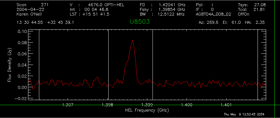
3.1.5 Process single on+off pair#
3.1.5.1 Process first polarization#
Process the first polarization of the on+off pair (scan #270, 271) using getps, setting the intensity unit to Jansky.
getps, 270, plnum=0, units='Jy'
The plotter should open and you should this spectrum:

3.1.5.2 Adjust x-axis#
Set the x-axis to an interesting frequency using setx:
setx, 1.396, 1.402

3.1.5.3 Accumulate results#
Accumulate the results from first polarization in the buffer using accum.
accum
3.1.5.4 Process second polarization#
Now process the second polarization of the same on+pff pair (scan #270, 271), again setting the intensity unit to Jansky.
getps, 270, plnum=1, units='Jy'
3.1.5.5 Accumulate results#
Accumulate the results from second polarization in the buffer.
accum
3.1.5.4 Average polarizations#
Using the function ave you can average the two polarizations (i.e. the two spectra you have just accumulated):
ave

3.1.6 Smooth the result#
Using gsmooth you can smooth your data. Here we also use the /decimate option, this will reduce the number of channels in your spectrum.
gsmooth, 100, /decimate

3.1.7 Fit the baseline#
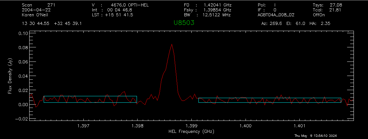
3.1.7.1 Choose region#
To choose the region for baseline fitting, use setregion and mark the start and end of the baseline region on either side of the source interactively. Use the left button of your mouse to mark the region and the right button to exit.
setregion
This is what the plotter window will look like after marking the basline regions (white vertical lines) while still in interactive more (green crosshair cursor).
This is what the plotter window will look like after exiting the interactive mode. The selected regions are now marked with the cyan rectangular boxes.
3.1.7.2 Set order of baseline fit#
We will use a polynomial baseline fit of order 3 (nfit).
nfit, 3
3.1.7.3 Show the fitted baseline#
Use bshape to show the fitted baseline
bshape
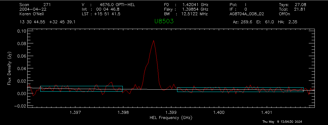
3.1.7.4 Subtract the fitted baseline#
To apply, i.e. subtract the fitted baseline from the data, use the command baseline:
baseline

3.1.8 Switch the x-axis#
Switch the x-axis from frequency to velocity (velo)
velo

3.1.9 Determine statistics#
3.1.9.1 RMS#
Determine the statistics (stats) in the velocity ranges surrounding the galaxy, i.e. 4000 km/s - 4400 km/s and 4800 km/s - 5200 km/s.
stats, 4000, 4400
    Chans    bchan    echan        Xmin        Xmax        Ymin        Ymax
       49      197      245      4003.4      4400.8  -0.0069890   0.0075569

                       Mean      Median         RMS    Variance        Area
                 1.9736E-06  0.00027831   0.0034322  1.1780E-05  0.00080165
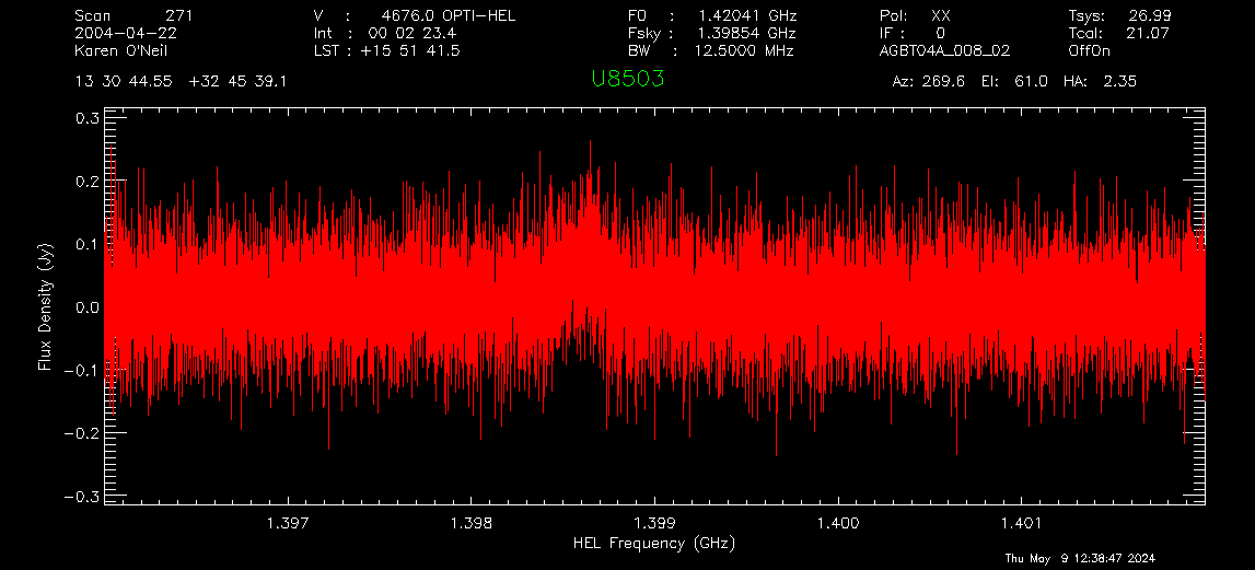
stats, 4800, 5200
    Chans    bchan    echan        Xmin        Xmax        Ymin        Ymax
       49      101      149      4799.2      5198.7  -0.0087689    0.011331

                       Mean      Median         RMS    Variance        Area
                -0.00011646 -0.00080158   0.0043761  1.9150E-05   -0.047555
3.1.9.2 Line properties#
Using the awv (area, width, velocity) routine, determine the line’s properties, including the velocity width at 20% of the line’s peak velocity.
gmeasure, 1, 0.2, brange=4610, erange=4735, rms=0.0039
Area, Width, Velocity (followed by errors in same order) = 3.67 83.31 4677.81 0.22 0.00 0.00
3.1.10 Compare with online database#
Check your results against the online database available here.
3.2 More Complicated Example#
This example is from the HI survey dataset.
It also matches the observation technique in Observing, example 1. Note, though, that not all the data in this dataset was taken using the standard ONOFF command with the cals (noise diodes) firing. Instead many of the observations were taken with the noise diodes turned off, followed by a short scan where the noise diodes are firing. As a result you need to determine the Tsys and then apply it to the on+off scans.
3.2.1 Start gbtidl#
Open a terminal. At the prompt enter
gbtidl
You should see the following welcome screen:
IDL Version 7.1.1 (linux x86_64 m64). (c) 2009, ITT Visual Information Solutions
Installation number: 15269-3.
Licensed for use by: National Radio Astronomy Observatory

Starting GBTIDL

Display Device  : X
Visual Class    : TrueColor
Visual Depth    : 24-Bit
Color Table Size: 256
Number of Colors: 16777216
Decomposed Color: 0

--------------------------------------------------------------------
                    Welcome to GBTIDL v2.10.1

    For news, documentation, enhancement requests, bug tracking,
               discussion, and contributions, visit:

                   http://gbtidl.nrao.edu

    For help with a GBTIDL routine from the command line, use
             the procedure 'usage'.  For example:

   usage,'show'           ; gives the syntax of the procedure 'show'
   usage,'show',/verbose  ; gives more information on 'show'
--------------------------------------------------------------------

GBTIDL ->
3.2.2 Load files of interest#
In GBTIDL use dirin to load the files you want to look at:
dirin, '/home/astro-util/HIsurvey/Session02'
3.2.3 Look at file content#
Using summary, you can get an overview of the content of the file you have just loaded:
summary
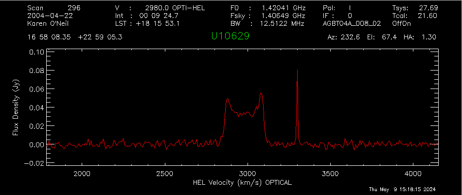
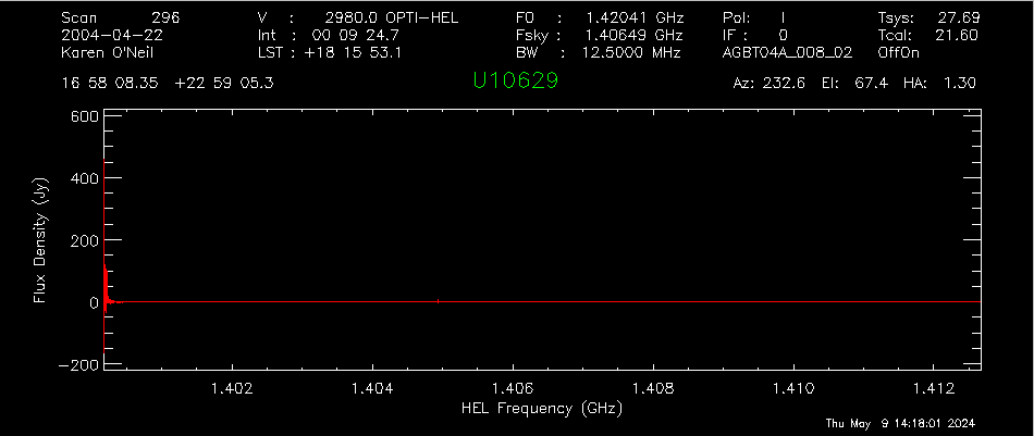
Here we’re showing only the scans of interest for this example. We have two OffOn pairs (scans pairs 295+296, 297+298) and one track scan (scan 299).
  Scan           Source      Vel    Proc Seq    RestF nIF nInt nFd     Az    El
   295           U10629   2980.0   OffOn   1    1.420   1   30   1  232.9  67.2
   296           U10629   2980.0   OffOn   2    1.420   1   30   1  232.6  67.4
   297           U10629   2980.0   OffOn   1    1.420   1   30   1  237.4  65.5
   298           U10629   2980.0   OffOn   2    1.420   1   30   1  237.1  65.6
   299           U10629   2980.0   Track   1    1.420   1    3   1  241.4  63.6
3.2.4 Double-check the scans#
list allows to list individual scans:
list, scan=295
Here you can see that there is no noise diode (cal) firing during the on + off scans. We’re only showing the first few lines of the output, when you run the command, the output list will be a bit longer.
 #INDEX           SOURCE       SCAN PROCEDURE POL IFNUM FDNUM        INT SIG CAL
   2472           U10629        295     OffOn  XX     0     0          0   T   F
   2473           U10629        295     OffOn  YY     0     0          0   T   F
   2474           U10629        295     OffOn  XX     0     0          1   T   F
   2475           U10629        295     OffOn  YY     0     0          1   T   F
   2476           U10629        295     OffOn  XX     0     0          2   T   F
   2477           U10629        295     OffOn  YY     0     0          2   T   F
   2478           U10629        295     OffOn  XX     0     0          3   T   F
   2479           U10629        295     OffOn  YY     0     0          3   T   F
   2480           U10629        295     OffOn  XX     0     0          4   T   F
   2481           U10629        295     OffOn  YY     0     0          4   T   F
list, scan=296
 #INDEX           SOURCE       SCAN PROCEDURE POL IFNUM FDNUM        INT SIG CAL
   2532           U10629        296     OffOn  XX     0     0          0   T   F
   2533           U10629        296     OffOn  YY     0     0          0   T   F
   2534           U10629        296     OffOn  XX     0     0          1   T   F
   2535           U10629        296     OffOn  YY     0     0          1   T   F
   2536           U10629        296     OffOn  XX     0     0          2   T   F
   2537           U10629        296     OffOn  YY     0     0          2   T   F
   2538           U10629        296     OffOn  XX     0     0          3   T   F
   2539           U10629        296     OffOn  YY     0     0          3   T   F
   2540           U10629        296     OffOn  XX     0     0          4   T   F
   2541           U10629        296     OffOn  YY     0     0          4   T   F
list, scan=299
 #INDEX           SOURCE       SCAN PROCEDURE POL IFNUM FDNUM        INT SIG CAL
   2712           U10629        299     Track  XX     0     0          0   T   T
   2713           U10629        299     Track  XX     0     0          0   T   F
   2714           U10629        299     Track  YY     0     0          0   T   T
   2715           U10629        299     Track  YY     0     0          0   T   F
   2716           U10629        299     Track  XX     0     0          1   T   T
   2717           U10629        299     Track  XX     0     0          1   T   F
   2718           U10629        299     Track  YY     0     0          1   T   T
   2719           U10629        299     Track  YY     0     0          1   T   F
   2720           U10629        299     Track  XX     0     0          2   T   T
   2721           U10629        299     Track  XX     0     0          2   T   F
   2722           U10629        299     Track  YY     0     0          2   T   T
   2723           U10629        299     Track  YY     0     0          2   T   F
3.2.5 Determine \(T_{sys}\)#
We will use the track scan (scan 299) to determine the system temperature, \(T_{sys}\) for each polarization. The procedure gettp allows us to load those scans:
gettp, 299, plnum=0
Scan: 299 (IF:0 FD:0 PL:0) Tsys: 27.98
gettp, 299, plnum=1
Scan: 299 (IF:0 FD:0 PL:1) Tsys: 27.40
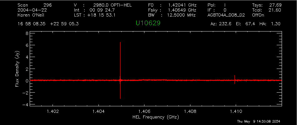
3.2.6 Empty the buffer memory#
Make sure the buffer memory is empty using sclear.
sclear
3.2.7 Process on+off pairs#
Here you have to use the getsigref command, and explicitly give the command the on and off scan numbers. We then use accum to accumulate the results for both polarizations and ave to average to accumulated spectra into one final spectra.
getsigref, 296, 295, plnum=0, tsys=27.98, unit='Jy'
SigScan: 296 RefScan: 295 (IF:0 FD:0 PL:0) units: Jy tau:0.008 ap_eff:0.710 Tsys: 27.98
accum
getsigref, 296, 295, plnum=1, tsys=27.40, unit='Jy'
Blanked spectra: ignored 2 integrations
SigScan:   296  RefScan:   295 (IF:0 FD:0 PL:1)   units: Jy  tau:0.008 ap_eff:0.710  Tsys:  27.40
accum
getsigref, 298, 297, plnum=0, tsys=27.98, unit='Jy'
SigScan: 298 RefScan: 297 (IF:0 FD:0 PL:0) units: Jy tau:0.008 ap_eff:0.710 Tsys: 27.98
accum
getsigref, 298, 297, plnum=0, tsys=27.40, unit='Jy'
SigScan: 298 RefScan: 297 (IF:0 FD:0 PL:1) units: Jy tau:0.008 ap_eff:0.710 Tsys: 27.40
accum
ave
3.2.8 Adjust x-axis#
Set the x-axis to avoid the edges (setx).
setx, 1.401, 1.412
3.2.9 Smooth the spectrum#
Using gsmooth you can smooth your data. Here we also use the /decimate option, this will reduce the number of channels in your spectrum.
gsmooth, 100, /decimate
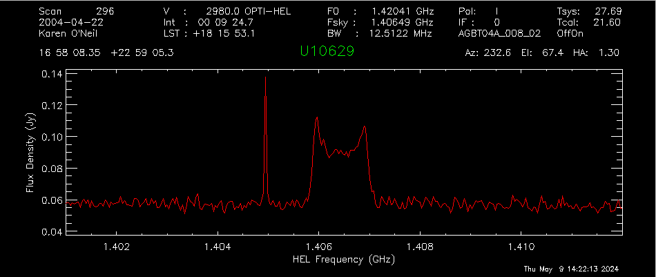
3.2.10 Remove baseline#
Set regions avoiding the RFI spike (setregion).
setregion

Remove baseline (after inspection) using first order polynomial (i.e. a line) using nfit, bshape, and baseline.
nfit, 1
GBTIDL -> bshape
GBTIDL -> baseline

3.2.11 Determine statistics#
3.2.11.1 RMS noise#
Determine the statistics in the velocity ranges surrounding the galaxy, i.e. 2000 km/s - 2500 km/s and 3500 km/s - 4000 km/s (stats).
stats, 2000, 2500
    Chans    bchan    echan        Xmin        Xmax        Ymin        Ymax
       63      222      284      1996.4      2503.1  -0.0050648   0.0063588

                       Mean      Median         RMS    Variance        Area
                 0.00022812  0.00011783   0.0025809  6.6610E-06     0.11764
stats, 3500, 4000
    Chans    bchan    echan        Xmin        Xmax        Ymin        Ymax
       62       40      101      3496.8      4000.3  -0.0062628   0.0065100

                       Mean      Median         RMS    Variance        Area
                -3.3634E-05 -0.00021309   0.0024638  6.0704E-06   -0.017239
3.2.11.2 Line properties#
Using the awv (area, width, velocity) routine, we can determine the line’s properties, including the velocity width at 20% of the line’s peak velocity. Here we will use a few methods:
-
- Fraction of mean
-
As a fraction of the mean within the region of interest. The mean of data from brange through erange is calculated. The edges are then those locations where the data values are greater than fract*mean for 3 consecutive channels starting from the end points of the region of interest and searching towards the center (method #1), first using 50% of the peak intensity and then 20%
gmeasure, 1, 0.5, brange=2815, erange=3142, rms=0.00252
Area, Width, Velocity (followed by errors in same order) = 9.45 252.76 2979.57 0.27 0.00 0.00
gmeasure, 1, 0.2, brange=2815, erange=3142, rms=0.00252
Area, Width, Velocity (followed by errors in same order) = 9.45 277.50 2974.64 0.26 0.00 0.00
-
- Fraction of maximum value
-
As a fraction of the maximum value within the region of interest. The peak of data from brange to erange is found. The edges are then those locations where the data values are greater than fract*(peak-rms) for 3 consecutive channels starting from the end points of the region of interest and searching towards the center (method #2) , first using 50% of the peak intensity and then 20%.
gmeasure, 2, 0.5, brange=2815, erange=3142, rms=0.00252
Area, Width, Velocity (followed by errors in same order) = 9.45 238.38 2980.15 0.26 0.00 0.00
gmeasure, 2, 0.2, brange=2815, erange=3142, rms=0.00252
Area, Width, Velocity (followed by errors in same order) = 9.45 258.82 2979.04 0.25 0.00 0.00
-
- Fraction of each of two peaks – identified by user
-
You use the cursor to mark two peaks in the region of interest or those peaks are identified through the lefthorn and righthorn parameters. The maximum value within 10 channels of each user-supplied peak location is found. The left edge is where the data value falls below fract*(peak-rms) for 3 consecutive channels searched from the location of the peak. The right-channel peak is similarly used to find the right edge (method #3) , first using 50% of the peak intensity and then 20%.
gmeasure, 3, 0.5, brange=2815, erange=3142, rms=0.00252
click on the positions for the two peaks
  Area, Width, Velocity (followed by errors in same order) =    9.49  239.90 2979.39    0.26    0.00    0.00
gmeasure, 3, 0.2, brange=2815, erange=3142, rms=0.00252
click on the positions for the two peaks
  Area, Width, Velocity (followed by errors in same order) =    9.49  259.96 2978.47    0.25    0.00    0.00
4. Data Reduction - scripted#
This example is from the HI survey dataset (http://greenbankobservatory.org/~koneil/HIsurvey/index.shtml).
You can download the example script shown below here:
HI_survey_process.pro
; Step 3.2.2
dirin,'/home/astro-util/HIsurvey/Session02'

jnk='jnk'   ; this is used later, to pause the observations
freeze      ; keep from plotting on the screen, to speed up the processing

; skipping steps 3.2.3, and 3.2.4 since you are running a script you should already understand your dataset.

; Steps 3.2.5  here we are running the commands quietly, and then
; getting the tsys values from the !g structure.

gettp,299,plnum=0, /quiet
tsys0=!g.s.tsys

gettp,299,plnum=1, /quiet
tsys1=!g.s.tsys

;Step 3.2.6 - clear the buffer
sclear

;Step 3.2.7; Here wer are going to loop over the scans of interest.
;Because this is a text file, we are using the $& at the end, to continue the lines
;appropriately.  Again this is being run quietly

for i=295,297,2 do begin &$  ; scan numbers
  for p=0,1 do begin &$      ; polarizzation numbers
    if (p eq 0) then tsys=tsys0[0] else tsys=tsys1[0] &$
    getsigref,i+1,i,plnum=p,tsys=tsys,unit='Jy', /quiet &$
    accum &$
  endfor &$
endfor

ave

; Step 3.2.8 - fix the x-axis
setxunit,'GHz' ; make sure we have the expected units in the x-axis.
setx,1.401,1.412

; Step 3.2.9 - smooth the data to the desired resolution
gsmooth,100,/decimate

show
unfreeze
; Step 3.2.10 - Remove baseline
; set region - Here we are going to avoid clicking on the screen and set the regions for the
; baseline fitting
region=[1.402, 1.4045, 1.40506, 1.4054, 1.4072, 1.4115]
reg1=xtochan(region)
Nregion,reg1
nfit,1
bshape

; this pauses the observations, to see the baseline shape
; this is only needed if this script is being read into gbtidl as a whole.
read,jnk,prompt='Push return to continue: '

;remove the baseline
baseline ; removes the baseline

; Step 3.2.11.1: determine (and print) the rms noise
velo
stats,2000,2500, ret=mystats
rms1 = mystats.rms
stats,3500,4000, ret=mystats
rms2 = mystats.rms

rms = (rms1 + rms2) / 2

; Step 3.2.11.2: determine the galaxy's mean intensity using method 1, and calculating the 20% and 50% velocity widths
gmeasure,1, 0.5,brange=2815,erange=3142,rms=rms
gmeasure,1, 0.2,brange=2815,erange=3142,rms=rms
- Let’s say you have the script saved as
HI_survey_process.pro. You can execute the script doing the following -
in a regular terminal
gbtidl
Within GBTIDL type
@HI_survey_process.pro
Once done you should see this output from the code:
% ACCUMAVE: Average of :           4 spectra
Push return to continue:
% Program caused arithmetic error: Floating divide by 0
    Chans    bchan    echan        Xmin        Xmax        Ymin        Ymax
       63      222      284      1996.4      2503.1  -0.0052186   0.0062189

                       Mean      Median         RMS    Variance        Area
                 8.7379E-05 -4.4913E-05   0.0025822  6.6675E-06    0.045062
    Chans    bchan    echan        Xmin        Xmax        Ymin        Ymax
       62       40      101      3496.8      4000.3  -0.0062437   0.0065244

                       Mean      Median         RMS    Variance        Area
                -1.8582E-06 -0.00018846   0.0024669  6.0857E-06 -0.00095242
  Area, Width, Velocity (followed by errors in same order) =    9.43  252.71 2979.58    0.27    0.00    0.00
  Area, Width, Velocity (followed by errors in same order) =    9.43  277.39 2974.65    0.26    0.00    0.00
As well as this spectrum in the GBTIDL Plotter (separate window)